Unit - 5
Graphs
A graph can be defined as group of vertices and edges that are used to connect these vertices. A graph can be seen as a cyclic tree, where the vertices (Nodes) maintain any complex relationship among them instead of having parent child relationship.
Definition
A graph G can be defined as an ordered set G (V, E) where V(G) represents the set of vertices and E(G) represents the set of edges which are used to connect these vertices.
Example
The following is a graph with 5 vertices and 6 edges.
This graph G can be defined as G = (V, E)
Where V = {A, B, C, D, E} and E = {(A, B), (A, C) (A, D), (B, D), (C, D), (B, E), (E, D)}.

Directed and Undirected Graph
A graph can be directed or undirected. However, in an undirected graph, edges are not associated with the directions with them. An undirected graph is shown in the above figure since its edges are not attached with any of the directions. If an edge exists between vertex A and B then the vertices can be traversed from B to A as well as A to B.
In a directed graph, edges form an ordered pair. Edges represent a specific path from some vertex A to another vertex B. Node A is called the initial node while node B is called terminal node.
A directed graph is shown in the following figure.
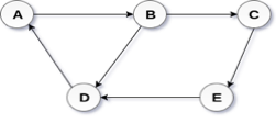
Fig 2– Directed graph
Graph Terminology
We use the following terms in graph data structure.
Vertex
Individual data element of a graph is called as Vertex. Vertex is also known as node. In above example graph, A, B, C, D & E are known as vertices.
Edge
An edge is a connecting link between two vertices. Edge is also known as Arc. An edge is represented as (startingVertex, endingVertex). For example, in above graph the link between vertices A and B is represented as (A, B). In above example graph, there are 7 edges (i.e., (A, B), (A, C), (A, D), (B, D), (B, E), (C, D), (D, E)).
Edges are three types.
- Undirected Edge - An undirected edge is a bidirectional edge. If there is undirected edge between vertices A and B then edge (A, B) is equal to edge (B, A).
- Directed Edge - A directed edge is a unidirectional edge. If there is directed edge between vertices A and B then edge (A, B) is not equal to edge (B, A).
- Weighted Edge - A weighted edge is an edge with value (cost) on it.
Undirected Graph
A graph with only undirected edges is said to be undirected graph.
Directed Graph
A graph with only directed edges is said to be directed graph.
Mixed Graph
A graph with both undirected and directed edges is said to be mixed graph.
End vertices or Endpoints
The two vertices joined by edge are called end vertices (or endpoints) of that edge.
Origin
If an edge is directed, its first endpoint is said to be the origin of it.
Destination
If an edge is directed, its first endpoint is said to be the origin of it and the other endpoint is said to be the destination of that edge.
Adjacent
If there is an edge between vertices A and B then both A and B are said to be adjacent. In other words, vertices A and B are said to be adjacent if there is an edge between them.
Incident
Edge is said to be incident on a vertex if the vertex is one of the endpoints of that edge.
Outgoing Edge
A directed edge is said to be outgoing edge on its origin vertex.
Incoming Edge
A directed edge is said to be incoming edge on its destination vertex.
Degree
Total number of edges connected to a vertex is said to be degree of that vertex.
Indegree
Total number of incoming edges connected to a vertex is said to be indegree of that vertex.
Outdegree
Total number of outgoing edges connected to a vertex is said to be outdegree of that vertex.
Parallel edges or Multiple edges
If there are two undirected edges with same end vertices and two directed edges with same origin and destination, such edges are called parallel edges or multiple edges.
Self-loop
Edge (undirected or directed) is a self-loop if its two endpoints coincide with each other.
Simple Graph
A graph is said to be simple if there are no parallel and self-loop edges.
Path
A path is a sequence of alternate vertices and edges that starts at a vertex and ends at other vertex such that each edge is incident to its predecessor and successor vertex.
Graph Representation
By Graph representation, we simply mean the technique which is to be used in order to store some graph into the computer's memory.
There are two ways to store Graph into the computer's memory.
1. Sequential Representation
In sequential representation, we use an adjacency matrix to store the mapping represented by vertices and edges. In adjacency matrix, the rows and columns are represented by the graph vertices. A graph having n vertices, will have a dimension n x n.
An entry Mij in the adjacency matrix representation of an undirected graph G will be 1 if there exists an edge between Vi and Vj.
An undirected graph and its adjacency matrix representation is shown in the following figure.

Fig: Undirected graph and its adjacency matrix
In the above figure, we can see the mapping among the vertices (A, B, C, D, E) is represented by using the adjacency matrix which is also shown in the figure.
There exists different adjacency matrices for the directed and undirected graph. In directed graph, an entry Aij will be 1 only when there is an edge directed from Vi to Vj.
A directed graph and its adjacency matrix representation is shown in the following figure.
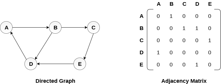
Fig- Directed graph and its adjacency matrix
Representation of weighted directed graph is different. Instead of filling the entry by 1, the Non- zero entries of the adjacency matrix are represented by the weight of respective edges.
The weighted directed graph along with the adjacency matrix representation is shown in the following figure.
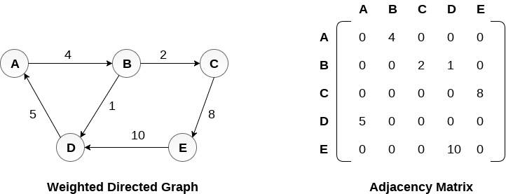
Fig - Weighted directed graph
2. Linked Representation
In the linked representation, an adjacency list is used to store the Graph into the computer's memory.
Consider the undirected graph shown in the following figure and check the adjacency list representation.

An adjacency list is maintained for each node present in the graph which stores the node value and a pointer to the next adjacent node to the respective node. If all the adjacent nodes are traversed then store the NULL in the pointer field of last node of the list. The sum of the lengths of adjacency lists is equal to the twice of the number of edges present in an undirected graph.
Consider the directed graph shown in the following figure and check the adjacency list representation of the graph.
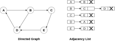
In a directed graph, the sum of lengths of all the adjacency lists is equal to the number of edges present in the graph.
In the case of weighted directed graph, each node contains an extra field that is called the weight of the node. The adjacency list representation of a directed graph is shown in the following figure.

Key takeaway
A graph can be defined as group of vertices and edges that are used to connect these vertices.
A graph can be seen as a cyclic tree, where the vertices (Nodes) maintain any complex relationship among them instead of having parent child relationship.
By Graph representation, we simply mean the technique which is to be used in order to store some graph into the computer's memory.
There are two ways to store Graph into the computer's memory.
We can represent a graph in matrix form in two ways-
1. Adjacent matrix
2. Incidence matrix
Adjacency matrix of a non-directed graph-
Let G be a graph with n vertices and no parallel edges. The adjacency matrix of G in a n × n. Symmetric binary matrix A (G) = [aij]nxn
Where


Where vi and vj are vertices of G.
The following is a example of the adjacency matrix of the simple graph G.
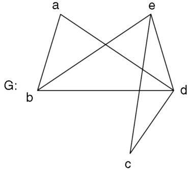
Adjacency matrix x; A (G)-
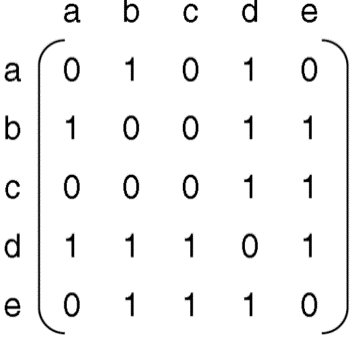
Adjacency matrix of a Digraph-
Let G be a digraph with n vertices, containing non-parallel edges. The adjacency matrix A(G) of the digraph G is an n × n matrix defined by


= 0 otherwise
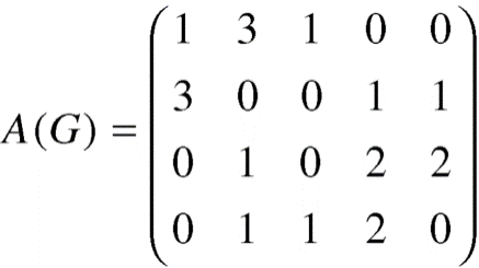
Example: Find the adjacency matrix of the graph-
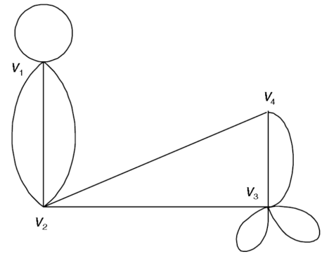
Sol. The adjacency matrix of the above graph will be-
Incidence matrix of a non-directed graph-
Let G be a graph with n vertices and m edges. The incidence matrix denoted by X (G) is defined as the matrix X (G) is defined as the matrix


= 0, otherwise
X (G) is an n by m matrix whose n rows correspond to the n vertices, and mcolumns correspond to m edges.
Graph and its incidence matrix-

Key takeaway
We can represent a graph in matrix form in two ways- 1. Adjacent matrix 2. Incidence matrix.
An adjacency list is used to store the Graph in the computer's memory in the linked representation.
Examine the adjacency list representation of the undirected graph depicted in the following image.

For each node in the graph, an adjacency list is kept, which contains the node value as well as a pointer to the node's next adjacent node. If all neighbouring nodes have been traversed, store NULL in the list's last node's pointer field. In an undirected graph, the sum of the lengths of adjacency lists is equal to twice the number of edges.
Examine the directed graph in the following graphic and look at the graph's adjacency list representation.
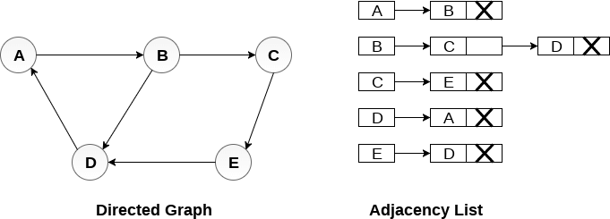
The total of the lengths of all the adjacency lists in a directed graph equals the number of edges in the graph.
In the case of a weighted directed graph, each node has an additional field called the node's weight. The following diagram depicts a directed graph's adjacency list representation.

A directed graph, also known as a digraph, is a graph with edges that have a certain direction. This is commonly represented by an arrow on the edge; more strictly, an edge is an unordered pair v,w if v and w are vertices, whereas a directed edge, called an arc, is an ordered pair (v,w) or (w,v) if v and w are vertices. The arc (v,w) is represented as an arrow pointing from v to w. Because the arcs (v,w) and (w,v) are separate, a graph with both arcs (v,w) and (w,v) is not a "multiple edge." Numerous arcs are possible, i.e., one arc (v,w) can appear in the multiset of arcs multiple times. If there are no loops or many arcs, a digraph is called simple.
The set of all arcs of the form (w,v) is denoted by Ev, and the set of arcs of the type (v,w) is denoted by E+v. The number of arcs in Ev is denoted by the indegree d(v), whereas the number of arcs in E+v is marked by the outdegree d+(v). The degrees are commonly denoted d1,d2,...,dn and d+1,d+2,...,d+n if the vertices are v1,v2,...,vn. Both ni=0di and ni=0d+i count the number of arcs exactly once, and ni=0di=ni=0d+i, of course. A digraph walk is a sequence of v1,e1,v2,e2,...,vk1,ek1,vk such that ek=(vi,vi+1); if v1=vk, it is a closed walk or a circuit. In a digraph, a path is a walk in which all of the vertices are distinct. It's not difficult to demonstrate that, in the case of graphs, if there's a walk from v to w, there's also a path from v to w.
Many of the issues we've looked at in graphs have analogues in digraphs, but there are also a lot of new ones. In the latter group, we'll look at one very significant outcome.
A network is a two-dimensional graph having a source s and a target ts. Each arc e also has a positive capacity, c(e).
Networks can be used to mimic the transmission of a physical quantity like oil or energy, or something more abstract like information, over a physical network.
A network flow is a function f from the digraph's arcs to R, with 0f(e)c(e) for all e, and such that
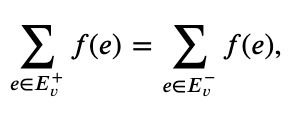
For all 𝑣 other than 𝑠 and 𝑡.
We want to give a flow a value that equals the net flow out of the source. Because the substance being transported cannot "collect" or "originate" at any vertex other than s and t, it appears logical to assume that this value likewise represents the net flow into the target.
We need to propose some new notation before we can verify this. Assume that U is a network's set of vertices, with 𝑠∈𝑈 and 𝑡∉𝑈. Let 𝑈→ be the set of arcs (𝑣,𝑤) with 𝑣∈𝑈, 𝑤∉𝑈, and 𝑈← be the set of arcs (𝑣,𝑤) with 𝑣∉𝑈, 𝑤∈𝑈.
Depth first search
Depth First Search is an algorithm for traversing or searching a graph.
It starts from some node as the root node and explores each and every branch of that node before backtracking to the parent node.
DFS is an uninformed search that progresses by expanding the first child node of the graph that appears and thus going deeper and deeper until a goal node is found, or until it hits a node that has no children.
Then the search backtracks, returning to the most recent node it hadn't finished exploring. In a non-recursive implementation, all freshly expanded nodes are added to a LIFO stack for expansion.
Steps for implementing Depth first search
Step 1: - Define an array A or Vertex that store Boolean values, its size should be greater or equal to the number of vertices in the graph G.
Step 2: - Initialize the array A to false
Step 3: - For all vertices v in G
If A[v] = false
Process (v)
Step 4: - Exit
Algorithm for DFS
DFS(G)
{
For each v in V, //for loop V+1 times
{
Color[v]=white; // V times
p[v]=NULL; // V times
}
Time=0; // constant time O (1)
For each u in V, //for loop V+1 times
If (color[u]==white) // V times
DFSVISIT(u) // call to DFSVISIT(v), at most V times O(V)
}
DFSVISIT(u)
{
Color[u]=gray; // constant time
t[u] = ++time;
For each v in Adj(u) // for loop
If (color[v] == white)
{
p[v] = u;
DFSVISIT(v); // call to DFSVISIT(v)
}
Color[u] = black; // constant time
f[u]=++time; // constant time
}
DFS algorithm used to solve following problems:
● Testing whether graph is connected.
● Computing a spanning forest of graph.
● Computing a path between two vertices of graph or equivalently reporting that no such path exists.
● Computing a cycle in graph or equivalently reporting that no such cycle exists.
Example:
Consider the graph G along with its adjacency list, given in the figure below. Calculate the order to print all the nodes of the graph starting from node H, by using depth first search (DFS) algorithm.
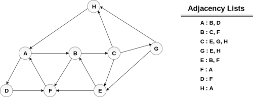
Solution:
Push H onto the stack
- STACK: H
POP the top element of the stack i.e. H, print it and push all the neighbours of H onto the stack that are is ready state.
- Print H
- STACK: A
Pop the top element of the stack i.e. A, print it and push all the neighbours of A onto the stack that are in ready state.
- Print A
- Stack: B, D
Pop the top element of the stack i.e. D, print it and push all the neighbours of D onto the stack that are in ready state.
- Print D
- Stack: B, F
Pop the top element of the stack i.e. F, print it and push all the neighbours of F onto the stack that are in ready state.
- Print F
- Stack: B
Pop the top of the stack i.e. B and push all the neighbours
- Print B
- Stack: C
Pop the top of the stack i.e. C and push all the neighbours.
- Print C
- Stack: E, G
Pop the top of the stack i.e. G and push all its neighbours.
- Print G
- Stack: E
Pop the top of the stack i.e. E and push all its neighbours.
- Print E
- Stack:
Hence, the stack now becomes empty and all the nodes of the graph have been traversed.
The printing sequence of the graph will be:
- H → A → D → F → B → C → G → E
Analysis of DFS
In the above algorithm, there is only one DFSVISIT(u) call for each vertex u in the vertex set V. Initialization complexity in DFS(G) for loop is O(V). In second for loop of DFS(G), complexity is O(V) if we leave the call of DFSVISIT(u).
Now, let us find the complexity of function DFSVISIT(u)
The complexity of for loop will be O(deg(u)+1) if we do not consider the recursive call to DFSVISIT(v). For recursive call to DFSVISIT(v), (complexity will be O(E) as
Recursive call to DFSVISIT(v) will be at most the sum of degree of adjacency for all vertex v in the vertex set V. It can be written as ∑ |Adj(v)|=O(E) vεV
The running time of DSF is (V + E).
Breadth first search
It is an uninformed search methodology which first expand and examine all nodes of graph systematically in search of the solution in the sequence and then go at the deeper level. In other words, it exhaustively searches the entire graph without considering the goal until it finds it.
From the standpoint of the algorithm, all child nodes obtained by expanding a node are added to a FIFO queue. In typical implementations, nodes that have not yet been examined for their neighbors are placed in some container (such as a queue or linked list) called "open" and then once examined are placed in the container "closed".
Steps for implementing Breadth first search
Step 1: - Initialize all the vertices by setting Flag = 1
Step 2: - Put the starting vertex A in Q and change its status to the waiting state by setting Flag = 0
Step 3: - Repeat through step 5 while Q is not NULL
Step 4: - Remove the front vertex v of Q. Process v and set the status of v to the processed status by setting Flag = -1
Step 5: - Add to the rear of Q all the neighbour of v that are in the ready state by setting Flag = 1 and change their status to the waiting state by setting flag = 0
Step 6: - Exit
Algorithm for BFS
BFS (G, s)
{
For each v in V - {s} // for loop {
Color[v]=white;
d[v]= INFINITY;
p[v]=NULL;
}
Color[s] = gray;
d[s]=0;
p[s]=NULL;
Q = ø; // Initialize queue is empty
Enqueue(Q, s); /* Insert start vertex s in Queue Q */
While Q is nonempty // while loop
{
u = Dequeue[Q]; /* Remove an element from Queue Q*/
For each v in Adj[u] // for loop
{ if (color[v] == white) /*if v is unvisted*/
{
Color[v] = gray; /* v is visted */
d[v] = d[u] + 1; /*Set distance of v to no. Of edges from s to u*/
p[v] = u; /*Set parent of v*/
Enqueue(Q,v); /*Insert v in Queue Q*/
}
}
Color[u] = black; /*finally visted or explored vertex u*/
}
}
Breadth First Search algorithm used in
● Prim's MST algorithm.
● Dijkstra's single source shortest path algorithm.
● Testing whether graph is connected.
● Computing a cycle in graph or reporting that no such cycle exists.
Example
Consider the graph G shown in the following image, calculate the minimum path p from node A to node E. Given that each edge has a length of 1.

Solution:
Minimum Path P can be found by applying breadth first search algorithm that will begin at node A and will end at E. The algorithm uses two queues, namely QUEUE1 and QUEUE2. QUEUE1 holds all the nodes that are to be processed while QUEUE2 holds all the nodes that are processed and deleted from QUEUE1.
Let’s start examining the graph from Node A.
1. Add A to QUEUE1 and NULL to QUEUE2.
QUEUE1 = {A}
QUEUE2 = {NULL}
2. Delete the Node A from QUEUE1 and insert all its neighbours. Insert Node A into QUEUE2
QUEUE1 = {B, D}
QUEUE2 = {A}
3. Delete the node B from QUEUE1 and insert all its neighbours. Insert node B into QUEUE2.
QUEUE1 = {D, C, F}
QUEUE2 = {A, B}
4. Delete the node D from QUEUE1 and insert all its neighbours. Since F is the only neighbour of it which has been inserted, we will not insert it again. Insert node D into QUEUE2.
QUEUE1 = {C, F}
QUEUE2 = { A, B, D}
5. Delete the node C from QUEUE1 and insert all its neighbours. Add node C to QUEUE2.
QUEUE1 = {F, E, G}
QUEUE2 = {A, B, D, C}
6. Remove F from QUEUE1 and add all its neighbours. Since all of its neighbours has already been added, we will not add them again. Add node F to QUEUE2.
QUEUE1 = {E, G}
QUEUE2 = {A, B, D, C, F}
7. Remove E from QUEUE1, all of E's neighbours has already been added to QUEUE1 therefore we will not add them again. All the nodes are visited and the target node i.e. E is encountered into QUEUE2.
QUEUE1 = {G}
QUEUE2 = {A, B, D, C, F, E}
Now, backtrack from E to A, using the nodes available in QUEUE2.
The minimum path will be A → B → C → E.
Analysis of BFS
In this algorithm first for loop executes at most O(V) times.
While loop executes at most O(V) times as every vertex v in V is enqueued only once in the Queue Q. Every vertex is enqueued once and dequeued once so queuing will take at most O(V) time.
Inside while loop, there is for loop which will execute at most O(E) times as it will be at most the sum of degree of adjacency for all vertex v in the vertex set V.
Which can be written as
∑ |Adj(v)|=O(E)
vεV
Total running time of BFS is O(V + E).
Like depth first search, BFS traverse a connected component of a given graph and defines a spanning tree.
Space complexity of DFS is much lower than BFS (breadth-first search). It also lends itself much better to heuristic methods of choosing a likely-looking branch. Time complexity of both algorithms are proportional to the number of vertices plus the number of edges in the graphs they traverse.
Key takeaways
- Depth First Search is an algorithm for traversing or searching a graph.
- DFS is an uninformed search that progresses by expanding the first child node of the graph that appears and thus going deeper and deeper until a goal node is found, or until it hits a node that has no children.
- BFS is an uninformed search methodology which first expand and examine all nodes of graph systematically in search of the solution in the sequence and then goes to the deeper level.
- In other words, it exhaustively searches the entire graph without considering the goal until it finds it.
Difference between DFS and BFS
| BFS | DFS |
Full form | BFS stands for Breadth First Search. | DFS stands for Depth First Search. |
Technique | It a vertex-based technique to find the shortest path in a graph. | It is an edge-based technique because the vertices along the edge are explored first from the starting to the end node. |
Definition | BFS is a traversal technique in which all the nodes of the same level are explored first, and then we move to the next level. | DFS is also a traversal technique in which traversal is started from the root node and explore the nodes as far as possible until we reach the node that has no unvisited adjacent nodes. |
Data Structure | Queue data structure is used for the BFS traversal. | Stack data structure is used for the BFS traversal. |
Backtracking | BFS does not use the backtracking concept. | DFS uses backtracking to traverse all the unvisited nodes. |
Number of edges | BFS finds the shortest path having a minimum number of edges to traverse from the source to the destination vertex. | In DFS, a greater number of edges are required to traverse from the source vertex to the destination vertex. |
Optimality | BFS traversal is optimal for those vertices which are to be searched closer to the source vertex. | DFS traversal is optimal for those graphs in which solutions are away from the source vertex. |
Speed | BFS is slower than DFS. | DFS is faster than BFS. |
Suitability for decision tree | It is not suitable for the decision tree because it requires exploring all the neighboring nodes first. | It is suitable for the decision tree. Based on the decision, it explores all the paths. When the goal is found, it stops its traversal. |
Memory efficient | It is not memory efficient as it requires more memory than DFS. | It is memory efficient as it requires less memory than BFS. |
A spanning tree is a subset of Graph G that covers all of the vertices with the fewest number of edges feasible. As a result, a spanning tree has no cycles and cannot be disconnected.
We can deduce from this definition that every linked and undirected Graph G contains at least one spanning tree. Because a disconnected graph cannot be spanned to all of its vertices, it lacks a spanning tree.
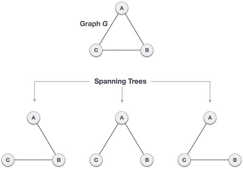
Fig: Spanning tree
From a single full graph, we discovered three spanning trees. The greatest number of spanning trees in a full undirected graph is nn-2, where n is the number of nodes. Because n is 3 in the example above, 33-2 = 3 spanning trees are conceivable.
Properties of spanning tree
We now know that a graph can contain many spanning trees. A few features of the spanning tree related to graph G are listed below.
● There can be more than one spanning tree in a linked graph G.
● The number of edges and vertices in all conceivable spanning trees of graph G is the same.
● There is no cycle in the spanning tree (loops).
● When one edge is removed from the spanning tree, the graph becomes unconnected, i.e. the spanning tree becomes minimally connected.
● When one edge is added to the spanning tree, a circuit or loop is created, indicating that the spanning tree is maximally acyclic.
Mathematical Properties of Spanning Tree
- Spanning tree has n-1 edges, where n is the number of nodes (vertices).
- From a complete graph, by removing maximum e - n + 1 edges, we can construct a spanning tree.
- A complete graph can have maximum nn-2 number of spanning trees.
Application of spanning tree
The spanning tree is used to discover the shortest path between all nodes in a graph. The use of spanning trees is common in a variety of situations.
● Civil Network Planning
● Computer Network Routing Protocol
● Cluster Analysis
Let's look at an example to help us comprehend. Consider the city network as a large graph, and the current objective is to deploy telephone lines in such a way that we can link to all city nodes with the bare minimum of lines. The spanning tree enters the scene at this point.
Key takeaway
- A spanning tree is a subset of Graph G that covers all of the vertices with the fewest amount of edges feasible.
- As a result, a spanning tree has no cycles and cannot be disconnected.
One of the searching techniques that requires a constant time is hashing. Hashing has an O time complexity (1). We've gone through the two types of search strategies so far: linear search and binary search. In linear search, the worst time complexity is O(n), whereas in binary search, it's O(logn). The quantity of components affects the search in both strategies, but we want a technique that takes a consistent amount of time. As a result, the hashing technique was developed, which gives a constant time.
The hash table and hash function are employed in the hashing technique. We can calculate the address at which the value can be stored using the hash function.
The primary goal of hashing is to generate (key/value) pairs. If the key is provided, the algorithm calculates the index where the value will be stored. It's possible to write it as:
Index = hash(key)
Consider an example of hash table of size 20, and the following items are to be stored. Item are in the (key,value) format.

● (1,20)
● (2,70)
● (42,80)
● (4,25)
● (12,44)
● (14,32)
● (17,11)
● (13,78)
● (37,98)
Sr.No. | Key | Hash | Array Index |
1 | 1 | 1 % 20 = 1 | 1 |
2 | 2 | 2 % 20 = 2 | 2 |
3 | 42 | 42 % 20 = 2 | 2 |
4 | 4 | 4 % 20 = 4 | 4 |
5 | 12 | 12 % 20 = 12 | 12 |
6 | 14 | 14 % 20 = 14 | 14 |
7 | 17 | 17 % 20 = 17 | 17 |
8 | 13 | 13 % 20 = 13 | 13 |
9 | 37 | 37 % 20 = 17 | 17 |
Linear Probing
As we can see, it may happen that the hashing technique is used to create an already used index of the array. In such a case, we can search the next empty location in the array by looking into the next cell until we find an empty cell. This technique is called linear probing.
Sr.No. | Key | Hash | Array Index | After Linear Probing, Array Index |
1 | 1 | 1 % 20 = 1 | 1 | 1 |
2 | 2 | 2 % 20 = 2 | 2 | 2 |
3 | 42 | 42 % 20 = 2 | 2 | 3 |
4 | 4 | 4 % 20 = 4 | 4 | 4 |
5 | 12 | 12 % 20 = 12 | 12 | 12 |
6 | 14 | 14 % 20 = 14 | 14 | 14 |
7 | 17 | 17 % 20 = 17 | 17 | 17 |
8 | 13 | 13 % 20 = 13 | 13 | 13 |
9 | 37 | 37 % 20 = 17 | 17 | 18 |
Hash table
A hash table is a type of data structure that employs a particular function known as a hash function to map a given value to a key in order to retrieve elements more quickly.
A hash table is a data structure that stores information with two major components: key and value. With the help of an associative array, a hash table can be created. The effectiveness of the hash function used for mapping is determined by the efficiency of the hash function used for mapping.
For example, if the key value is John and the value is the phone number, we may use the following hash function to pass the key value:
Hash(key)= inex;
The index is returned when the key is passed to the hash function.
Hash(john) = 3;
The john is added to the index 3 in the example above.
Basic Operations
Following are the basic primary operations of a hash table.
- Search − Searches an element in a hash table.
- Insert − inserts an element in a hash table.
- Delete − Deletes an element from a hash table.
Data Item
Define a data item having some data and key, based on which the search is to be conducted in a hash table.
Struct DataItem {
Int data;
Int key;
};
Hash Method
Define a hashing method to compute the hash code of the key of the data item.
Int hashCode(int key){
Return key % SIZE;
}
Search Operation
Whenever an element is to be searched, compute the hash code of the key passed and locate the element using that hash code as index in the array. Use linear probing to get the element ahead if the element is not found at the computed hash code.
Example
Struct DataItem *search(int key) {
//get the hash
Int hashIndex = hashCode(key);
//move in array until an empty
While(hashArray[hashIndex] != NULL) {
If(hashArray[hashIndex]->key == key)
Return hashArray[hashIndex];
//go to next cell
++hashIndex;
//wrap around the table
HashIndex %= SIZE;
}
Return NULL;
}
Insert Operation
Whenever an element is to be inserted, compute the hash code of the key passed and locate the index using that hash code as an index in the array. Use linear probing for empty location, if an element is found at the computed hash code.
Example
Void insert(int key,int data) {
Struct DataItem *item = (struct DataItem*) malloc(sizeof(struct DataItem));
Item->data = data;
Item->key = key;
//get the hash
Int hashIndex = hashCode(key);
//move in array until an empty or deleted cell
While(hashArray[hashIndex] != NULL && hashArray[hashIndex]->key != -1) {
//go to next cell
++hashIndex;
//wrap around the table
HashIndex %= SIZE;
}
HashArray[hashIndex] = item;
}
Delete Operation
Whenever an element is to be deleted, compute the hash code of the key passed and locate the index using that hash code as an index in the array. Use linear probing to get the element ahead if an element is not found at the computed hash code. When found, store a dummy item there to keep the performance of the hash table intact.
Example
Struct DataItem* delete(struct DataItem* item) {
Int key = item->key;
//get the hash
Int hashIndex = hashCode(key);
//move in array until an empty
While(hashArray[hashIndex] !=NULL) {
If(hashArray[hashIndex]->key == key) {
Struct DataItem* temp = hashArray[hashIndex];
//assign a dummy item at deleted position
HashArray[hashIndex] = dummyItem;
Return temp;
}
//go to next cell
++hashIndex;
//wrap around the table
HashIndex %= SIZE;
}
Return NULL;
}
Hash Table Program in C
Hash Table is a data structure which stores data in an associative manner. In hash table, the data is stored in an array format where each data value has its own unique index value. Access of data becomes very fast, if we know the index of the desired data.
Implementation in C
#include <stdio.h>
#include <string.h>
#include <stdlib.h>
#include <stdbool.h>
#define SIZE 20
Struct DataItem {
Int data;
Int key;
};
Struct DataItem* hashArray[SIZE];
Struct DataItem* dummyItem;
Struct DataItem* item;
Int hashCode(int key) {
Return key % SIZE;
}
Struct DataItem *search(int key) {
//get the hash
Int hashIndex = hashCode(key);
//move in array until an empty
While(hashArray[hashIndex] != NULL) {
If(hashArray[hashIndex]->key == key)
Return hashArray[hashIndex];
//go to next cell
++hashIndex;
//wrap around the table
HashIndex %= SIZE;
}
Return NULL;
}
Void insert(int key,int data) {
Struct DataItem *item = (struct DataItem*) malloc(sizeof(struct DataItem));
Item->data = data;
Item->key = key;
//get the hash
Int hashIndex = hashCode(key);
//move in array until an empty or deleted cell
While(hashArray[hashIndex] != NULL && hashArray[hashIndex]->key != -1) {
//go to next cell
++hashIndex;
//wrap around the table
HashIndex %= SIZE;
}
HashArray[hashIndex] = item;
}
Struct DataItem* delete(struct DataItem* item) {
Int key = item->key;
//get the hash
Int hashIndex = hashCode(key);
//move in array until an empty
While(hashArray[hashIndex] != NULL) {
If(hashArray[hashIndex]->key == key) {
Struct DataItem* temp = hashArray[hashIndex];
//assign a dummy item at deleted position
HashArray[hashIndex] = dummyItem;
Return temp;
}
//go to next cell
++hashIndex;
//wrap around the table
HashIndex %= SIZE;
}
Return NULL;
}
Void display() {
Int i = 0;
For(i = 0; i<SIZE; i++) {
If(hashArray[i] != NULL)
Printf(" (%d,%d)",hashArray[i]->key,hashArray[i]->data);
Else
Printf(" ~~ ");
}
Printf("\n");
}
Int main() {
DummyItem = (struct DataItem*) malloc(sizeof(struct DataItem));
DummyItem->data = -1;
DummyItem->key = -1;
Insert(1, 20);
Insert(2, 70);
Insert(42, 80);
Insert(4, 25);
Insert(12, 44);
Insert(14, 32);
Insert(17, 11);
Insert(13, 78);
Insert(37, 97);
Display();
Item = search(37);
If(item != NULL) {
Printf("Element found: %d\n", item->data);
} else {
Printf("Element not found\n");
}
Delete(item);
Item = search(37);
If(item != NULL) {
Printf("Element found: %d\n", item->data);
} else {
Printf("Element not found\n");
}
}
If we compile and run the above program, it will produce the following result −
Output
~~ (1,20) (2,70) (42,80) (4,25) ~~ ~~ ~~ ~~ ~~ ~~ ~~ (12,44) (13,78) (14,32) ~~ ~~ (17,11) (37,97) ~~
Element found: 97
Element not found
Searching Techniques of hash table
In data structures,
● There are several searching techniques like linear search, binary search, search trees etc.
● In these techniques, time taken to search any particular element depends on the total number of elements.
Example-
● Linear search takes O(n) time to perform the search in unsorted arrays consisting of n elements.
● Binary Search takes O(logn) time to perform the search in sorted arrays consisting of n elements.
● It takes O(logn) time to perform the search in BST consisting of n elements.
Drawback-
The main drawback of these techniques is-
● As the number of elements increases, time taken to perform the search also increases.
● This becomes problematic when total number of elements become too large.
Hashing in Data Structure-
In data structures,
● Hashing is a well-known technique to search any particular element among several elements.
● It minimizes the number of comparisons while performing the search.
Advantage-
Unlike other searching techniques,
● Hashing is extremely efficient.
● The time taken by it to perform the search does not depend upon the total number of elements.
● It completes the search with constant time complexity O(1).
The Hash Function is used to index the original value or key, and it is then utilized to obtain the data associated with the value or key. As a result, hashing is always a one-way process. By studying the hashed values, there is no need to "reverse engineer" the hash algorithm.
There are various types of hash functions available such as-
- Mid Square Hash Function
- Division Hash Function
- Folding Hash Function etc
It depends on the user which hash function he wants to use.
Properties of Hash Function-
The properties of a good hash function are-
● It is efficiently computable.
● It minimizes the number of collisions.
● It distributes the keys uniformly over the table.
Characteristics of good Hash Function
- The hash value is fully determined by the data being hashed.
- The hash Function uses all the input data.
- The hash function "uniformly" distributes the data across the entire set of possible hash values.
- The hash function generates complicated hash values for similar strings.
Some hash function
1. Division Method:
Choose a number m smaller than the number of n of keys in k (The number m is usually chosen to be a prime number or a number without small divisors, since this frequently a minimum number of collisions).
The hash function is:

For Example: if the hash table has size m = 12 and the key is k = 100, then h (k) = 4. Since it requires only a single division operation, hashing by division is quite fast.
2. Multiplication Method:
The multiplication method for creating hash functions operates in two steps. First, we multiply the key k by a constant A in the range 0 < A < 1 and extract the fractional part of kA. Then, we increase this value by m and take the floor of the result.
The hash function is:

Where "k A mod 1" means the fractional part of k A, that is, k A -⌊k A⌋.
3. Mid Square Method:
The key k is squared. Then function H is defined by
H (k) = L
Where L is obtained by deleting digits from both ends of k2. We emphasize that the same position of k2 must be used for all of the keys.
4. Folding Method:
The key k is partitioned into a number of parts k1, k2.... kn where each part except possibly the last, has the same number of digits as the required address.
Then the parts are added together, ignoring the last carry.
H (k) = k1+ k2+.....+kn
Example: Company has 68 employees, and each is assigned a unique four- digit employee number. Suppose L consist of 2- digit addresses: 00, 01, and 02....99. We apply the above hash functions to each of the following employee numbers:
- 3205, 7148, 2345
(a) Division Method: Choose a Prime number m close to 99, such as m =97, Then
- H (3205) = 4, H (7148) = 67, H (2345) = 17.
That is dividing 3205 by 17 gives a remainder of 4, dividing 7148 by 97 gives a remainder of 67, dividing 2345 by 97 gives a remainder of 17.
(b) Mid-Square Method:
k = 3205 7148 2345
k2= 10272025 51093904 5499025
h (k) = 72 93 99
Observe that fourth & fifth digits, counting from right are chosen for hash address.
(c) Folding Method: Divide the key k into 2 parts and adding yields the following hash address:
- H (3205) = 32 + 50 = 82 H (7148) = 71 + 84 = 55
- H (2345) = 23 + 45 = 68
Key takeaway
The Hash Function is used to index the original value or key, and it is then utilized to obtain the data associated with the value or key.
As a result, hashing is always a one-way process.
Hashing is implemented using one of two methods:
● Hashing with Chaining
● Hashing with open addressing
Hashing with chaining
The element in S is stored in Hash table T [0...m-1] of size m, where m is somewhat greater than n, the size of S, in Hashing with Chaining. There are m slots in the hash table. A hash function h is associated with the hashing technique, and it maps from U to {0...m-1}. We say that k is hashed into slot h since each key k ∈ S is kept in location T [h (k)] (k). A collision occurs when more than one key in S is hashed into the same slot.
All keys that hash into the same slot are placed in a linked list associated with that slot, which is referred to as the chain at slot. A hash table's load factor is defined as ∝=n/m, which represents the average amount of keys per slot. Because we frequently work in the m=θ(n) range, ∝ is usually a constant of ∝<1.
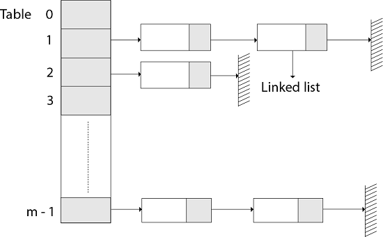
Fig: Hashing with chaining
Hashing with open address
All components in Open Addressing are kept in the hash table. That is, each table entry contains a dynamic set component or NIL. When looking for anything, we check table slots until we either find the item or establish that it isn't in the table. As a result, the load factor in open addressing can never exceed 1.
Open addressing has the advantage of avoiding Pointer. We compute the sequence of slots to be examined in this step. Because no pointers are shared, the hash table can have a larger number of slots for the same amount of memory, potentially resulting in fewer collisions and faster retrieval.
Probing is the process of inspecting a position in the hash table.
As a result, the hash function is transformed.
h : U x {0,1,....m-1} → {0,1,....,m-1}.
With open addressing, we need the probe sequence for every key k.
{h, (k, 0), h (k, 1)....h (k, m-1)}
Be a Permutation of (0, 1...... m-1)
A hash table T and a key k are passed to the HASH-INSERT method as inputs.
HASH-INSERT (T, k)
1. i ← 0
2. Repeat j ← h (k, i)
3. If T [j] = NIL
4. Then T [j] ← k
5. Return j
6. Else ← i= i +1
7. Until i=m
8. Error "hash table overflow"
The procedure HASH-SEARCH takes a hash table T and a key k as input and returns j if key k is found in slot j or NIL if key k is not found in table T.
HASH-SEARCH.T (k)
1. i ← 0
2. Repeat j ← h (k, i)
3. If T [j] =j
4. Then return j
5. i ← i+1
6. Until T [j] = NIL or i=m
7. Return NIL
Collision resolution strategies are divided into two categories.
● Separate chaining (open hashing)
● Open addressing (closed hashing)
Separate chaining
This strategy involves creating a linked list from the slot where the collision occurred, then inserting the new key into the linked list. Separate chaining refers to the linked list of slots that resembles a chain. When we don't know how many keys to insert or remove, we use it more.
Time complexity
● Its worst-case searching complexity is o (n).
● Its worst-case deletion complexity is o (n).
Advantages of separate chaining
● It is simple to put into practice.
● We can add more elements to the chain because the hash table never fills up.
● It is less sensitive to the hashing function.
Disadvantages of separate chaining
● Chaining cache performance is poor in this case.
● In this strategy, there is far too much memory waste.
● It necessitates a larger amount of space for element linkages.
Open addressing
Open addressing is a collision-resolution technique for preventing collisions in hashing tables. Outside of the hash table, no key is stored. As a result, the hash table's size is always more than or equal to the number of keys. Closed hashing is another name for it.
In open addressing, the following strategies are used:
● Linear probing
● Quadratic probing
● Double hashing
Key takeaway
The hash function is utilized to find the array's index in this case.
The hash value is used as an index in the hash table to hold the key.
For two or more keys, the hash function can return the same hash value.
When the home bucket for a new pair (key, element) is full, an overflow occurs.
We may tackle overflows by
Look through the hash table in a systematic manner for an empty bucket.
● Linear probing (linear open addressing).
● Quadratic probing.
● Random probing.
Allow each bucket to preserve a list of all pairings for which it is the home bucket to avoid overflows.
● Array linear list.
● Chain.
Open addressing is used to ensure that all elements are placed directly in the hash table, and it uses a variety of approaches to resolve collisions.
To resolve collisions, Linear Probing is used to place the data into the next available space in the table.
Performance of Linear Probing
● The worst-case time for find/insert/erase is (m), where m is the number of pairings in the table.
● When all pairings are in the same cluster, this happens.
Problem of Linear Probing
● Identifiers have a tendency to group together.
● Adjacent clusters are forming a ring.
● Increase or improve the time spent searching.
Quadratic Probing
Linear probing searches buckets (H(x)+i2)%b; H(x) indicates Hash function of x
Quadratic probing implements a quadratic function of i as the increment
Examine buckets H(x), (H(x)+i2)%b, (H(x)-i2)%b, for 1<=i<=(b-1)/2
b is indicated as a prime number of the form 4j+3, j is an integer
Random Probing
Random Probing performs incorporating random numbers.
H(x):= (H’(x) + S[i]) % b
S[i] is a table along with size b-1
S[i] is indicated as a random permutation of integers [1, b-1].
References:
- Aaron M. Tenenbaum, Yedidyah Langsam and Moshe J. Augenstein, “Data Structures Using C and C++”, PHI Learning Private Limited, Delhi India
- Horowitz and Sahani, “Fundamentals of Data Structures”, Galgotia Publications Pvt Ltd Delhi India.
- Lipschutz, “Data Structures” Schaum’s Outline Series, Tata McGraw-hill Education (India) Pvt. Ltd.
- Thareja, “Data Structure Using C” Oxford Higher Education.
- AK Sharma, “Data Structure Using C”, Pearson Education India.