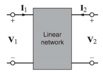
Unit - 5
Two port networks and Network functions
The parameters of a two- port network is called as two port network parameters. The types are: -
- Z parameters
- Y parameters
- T parameters
- T’ parameters
- h-parameters
- g-parameters
Z parameters:
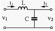
The following set of two equations by considering variables V1 & V2 as dependent and I1 & I2 as independent. The coefficients of independent variables, I1 and I2 are called as Z parameters.
V1 = Z11 I1 + Z12 I2
V2 = Z21 I1 + Z22 I2
The Z parameters are:
Z11 = V1 I1 when I2 =0
Z12 = V1 I2 when I1=0
Z21= V2I1 when I2 =0
Z22 = V2I1 when I2 =0
The Z parameters are called as impedance parameters because these are the ratio of volatges and currents.
To calculate Z11 and Z21 by doing open circuit of port2. Similiarly the other two parameters Z12 and Z22 are calculated by doing open circuit of port1.
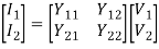
Y parameters:
The set of equations can be obtained by considering I1 and I2 as dependent and V1 and V2 as independent. The co-effecients of independent variables V1 and V2 are called as Y parameters.
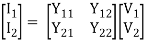
I1 = Y11 V1 + Y12 V2
I2 = Y21 V1 + Y22 V2
Y parameters are called as admittance parameters because these are simply, the ratios of currents and voltages. Units of Y parameters are mho.
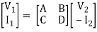
T parameters:
The set of equations can be obtained by considering V1 and I1 as dependent and V2 and I2 as independent. The coefficients V2 and I2 are called as T parameters.
V1 = A V2 – B I2
I1 = C V2 – D I2
The T parameters are :
A = V1/V2 when I2 =0
B = -V1 / I2 when V2 =0
C = I1/V2 when I2 =0
D = -I1/I2 when V2 =0
h- parameters
The following set of two equations by considering the variables V1 and I2 as dependent and I1 and V2 as independent. The coefficient of independent variables I1 and V2 are called as h-parameters.
V1 = h11 I1 + h12 V2
I2 = h21 I1 + h22 V2
The h parameters are:
h 11 = V1/I1 when V2 =0
h 12 = V1 / V2 when I1=0
h21 = I2/I1 when V2 =0
h22 = I2/V2 when I1 =0
h-parameters are called as hybrid parameters. The parameters, h12 and h21, do not have any units, since those are dimension-less. The units of parameters, h11 and h22, are Ohm and Mho respectively.
g-parameters
The following set of two equations can be obtained by considering the variables I1 & V2 as dependent and V1 & I2 as independent. The coefficients of independent variables, V1 and I2 are called as g-parameters.
I1=g11V1+g12I2I1
V2=g21V1+g22I2
The g-parameters are
g11=I1V1, whenI2=0
g12=I1I2, whenV1=0
g21=V2V1, whenI2=0
g22=V2I2, whenV1=0
g-parameters are called as inverse hybrid parameters.
Finding the model parameters
For each of the four types of models, the four parameters can be found from variables V1, V2 , I1,I2 network by the following.
- For Z-model:

- For Y-model:

- For A-model

- For H model

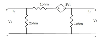
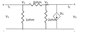
Find the Z-model and Y-model of the circuit
First assume I2 , we get
Assume I1 =0 we get
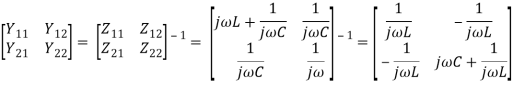
The parameters of the Y-model can be found as the inverse of:
Relation between Two- Port Parameters:
Δ = X11 X22 – X12 X21 ,ΔT = AD – BC
| [z] | [y] | [h] | [T] |
[z] | Z11 Z12 | 
|  |  |
Z21 Z22 |  | 
|  | |
|
|
|
|
|
[y] | 
| y11 y12 | 
|  |
 | y21 y22 |  | 
| |
|
|
|
|
|
[h] |  | 
| h11 h12 |  |
 |  | H21 h22 |  | |
[T] |  |  | 
| A B |

| 
|  | C D |
Driving point impedance
The driving point impedance is given for a two port network as
v1 = Z11I1 + Z12I2
v2 = Z11I1 + Z22I2
Z11 =  2=0
2=0
Z12 =  1=0
1=0
Z21 =  I2=0
I2=0
Z22 =  1=0
1=0
→I1 and I2 are excitations at port 1 & 2 respectively.
→V1 and V2 are the responses at port 1 and 2 respectively.
Driving point admittance
The driving point admittance for two port network function will be
I1 = Y11V1 + Y12V2
I2 = Y21V1 + Y22V2
Y11 =  V2=0
V2=0
Y12 =  V1=0
V1=0
Y21 =  V2=0
V2=0
Y22 =  V1=0
V1=0
V1& V2 should be independent
Their properties and concept of transfer impedance
Pole -Zero plot of a Network Function-
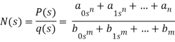
a, b- coefficient with are real and positive
Features of poles and zero of network function.
a) The network function is described by poles and zeros.
b) The zeros of the network exit for the complex frequencies where N(s)=0
c) The poles of the network exit for the complex frequencies where N(s)=o
d)The number of poles is equal to number of zeros considering types poles and zeros which at infinity.
e) when n>m, poles at infinity has degree(n-m)
f) When m>n, zeros at infinity with degree (m-n)
g) The time variation response of the network is determined through the poles.
h) The magnitude of response is determined by poles and zeros of the network function.
i) If q(s) =0, is the characteristics equation of N(S).
J) Capacitor is represented as (ʊ)=1/cs so, for
S = 0, It behaves open circuits
S=∞ behaves as short circuit
k) for inductor z(s) = Ls so, for
s= o It behaves short circuit
s =∞ It behaves as given circuits
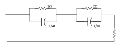
Que) For the network shown, find driving point input impedance. Plot the pole zero pattern for each as well.
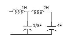
Solution- for fig 1) taking L.T we have
Z11= 1+ 1 /S/3+1/25+1/1/4S
=1+ 1/ 5/3+1/6S
=1+ 18S/6S2+3
Z11=6S2+3+18S/ 6S2+3 =2S2+6S+2/2S2+1
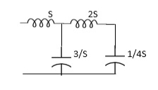
Zeros of equations are taking lt.of circuit b)
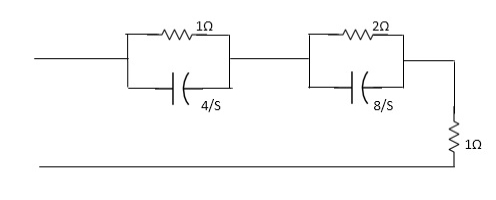
Z11= 1*4/5
1+4/5+2.8/3/2+8/5+1
=4/5+4 + 16/ 25+8+1
= 4/5+4+8/5+4+1
=s+12+4/ (5+4)
Z11= S+16/(S+4)
For zeros of system
s+16=0
s=-16
For poles of system
s+4=0
s=-4
Restrictions of poles and zeros on driving point function
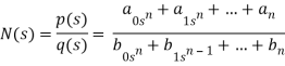
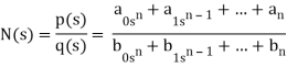
N(s) =p(s) =qosn+q, sn--------an/ q(s) bosn+b,sn-----------bn
1) All coefficient of p(s) and q(s) should be real and positive
2) poles and zeros must be conjugal whether imaginary or complex
3) Real part of poles and zeros must be negative or zero.
4) The degree of p(s) may differ either by zero or 1.
5) Lowest degree of p(s) and q(s) may differ at the most by one.
6) p(s) and q(s) cannot miss terms between highest and lowest degree unless all when or all odd terms are missing.
Q) Find whether the following network function represent the driving point function.
a) f(s)= (s+1)/(s2+1) b) f(s) = 3s2+2s+1/ss3+9s2+3s+2 c) f(s)=(s2+1)2/s2(s+3)
Solution
a) f(s)=s+1/s2+1
It represents the driving point function:
b) F(S)= 3S2+2S+1 / 5S3+9S2+3S+2
It represents the driving point function.
b) F(s)=3s2+2s+1/5s3+9s2+3s+2
It represents the driving point function
c) f(s) = (s2+1)2/s2(5+3)
It has representative zeros, hence not valid
(s2+1)2=0
s2=+-1
s2=+-j, +-j
v) Restriction as transfer function-
a) All coefficients of p(s) and q(s) should be real and positive for q(s)
b) The polis must be conjugal if imaginary or complex.
c) The real part of poles must be negative or new of zero than pole must be simple.
d)The degree of p(s) could be zero and it is independent of q(s). For example, f(s) 5/ (s3+3s+1)
e) q(s) cannot have missing terms between the highest and lowest degree unless all the even or all odd terms are missing
f) degree of q(s) >, p(s)
g) p(s) may have missing terms between the highest and lowest degree and its coefficients could be negative.
Time Domain Behaviour from pole -zero plot: -
To find the time domain behaviour we consider a simple RLC circuit. When the poles and zeros of I(s) can be represented in terms of undammed nautical frequency (wn)and damping ratio (ε). these can be represented as.
Wn = 1/√Lc and ε=R/2√C/L
For RLC network the characteristics equation of any second differential equation.
s2+2ε wns+wn2=0
s1s2=-2εwn+ 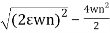
=-2εwn+ -
-
=-2εwn+ -
-
=-2εwn+-2
s1,s2 =-εwn+-wn 
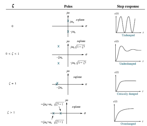
So, depending an § poles can be represented in various ways
a)ε>1
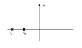
s1s2 = -εwn+- wn
As s1 s2 lies on negative real ax is .this corresponds to OVERDAMPED are have exponential decay from in the time domain.
b) 0<ε<1
s1s2 = -εwn+-∫wn
The roals are plotted below having both real and imaging part
1) Roals plot 2) Time response
As the roals have real and imaginary component as roals 0, this corresponds to UNDERDAMPED association. As initially oscillations exist but oscillations seen as t-∞
c)ε=0
s1s2 = -εwn+- wn
s2+2ε wns+w2n=0
For ε=0
s2+wn2=0
s=Ijwn
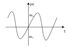
As the complex conjugal the as at t=0 and t=∞ same so, this is the case of UNDAMPED associations.
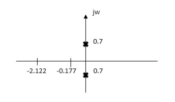
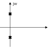
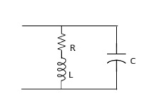
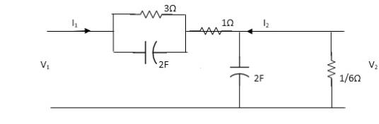
Q. For network below 1), pole - zero pattern is represented in fig 2, find numerical value of R,L and c for z (0)=1?
Solution
Calculating z(s) by taking L.T of fig 1)
z(s) = (R+SL) *1/CS
(R+SL)+1/CS = R+SL / SRC+S2LC+1
Z(S)= S+R/L / C [S2+R/L S+1/LC]
Given z (0) =1
z (0) =R/L / C/LC =1
Z (0) =R=1
.: R=1Ω
Polls are given as
S2+RS/L+1/LC=0
S=-R/2L +J
Zeros are given as
S+R / L=0
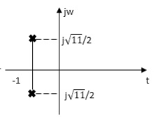
From pole zero plot value of pole location is at -1 so
-R / L = -1
-1/ L=-1
L=1H
Also, imaginary part of pole from plot is
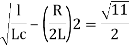
1/LC-(R/2L)2 =11/4
1/C-(1/2)2=11/4
1/C-1/4=11/4
1/C=11/4+1/4
1/C=12/4 =3
C=1/3 F
Hence, value of R=1Ω, L=14 and c=1/3 f
Q. FOR the following circuits, FIND G12(S) =v2/v1
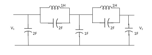
Solution: Taking Laplace transform of above we have
Applying KCL at node v0
V0-V1(S) / S*1/2S/(S+1/2S) +V0+V2(S)/ (S*1/2S)/(S+1/2S)+V0/1/S=0
For Porr 2) We have,
v2-v0/(s*1/2s)/(s+1/2s) +v2/1/s =0 ---------(ii)
(v2-v0) (2s2+1) / s +sv2=0
v2 [2s2+1/s+s] = v0(2s2+1)/ s
v0=v2(3s2+1) / (2s2+1) -----------(iii)
From (I) we have,
(v0-v1) /s (2s2+1) *sv0+(v0-v2)/5 (s2+1) =0
(2s2+1/5) v0-(2s2+1)/sv1+sv0+(2s2+1)/sv0-(s2+1)/s v2=0
(2s2+1)v1=(5s2+2)v0-(2s2+1)v2
Substitute value v0 from (iii) above
(2s2+1)v1 =[( 5s2+2)(3s2+1) /(2s2+1)-(2s2+1)]v2
(2s2+1)v1=(15s4+5s2+6s2+2-4s4+4s2) / (2s2+1 *v2
G12(s) = v2/v1 = (2s2+1) 2/11s4+15s2+1
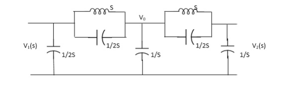
Q) Find the transfer function admittance ratio
Y12(s) = I2(S) / V1(S)
Solution:
Taking Laplace transform of above figure
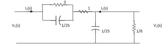
Applying KCL we get,
(V2-V1) / (3*1/2S) / (3+1/2S) * V2/ 1/2S+ V2/1/6 =0
(Y2-V1)(6S+1) / (6S+4) * (2S+6)V2V=0
BUT I2=-6V2
V2=-I2/6
We have,
(6s+1) / (6s+4)*v2-(6s+1) / (6s+4)*v1 +(2s+6)v2=0
-[6s+1 / 6s+s+2s+6]I2 / 6 =V1(6S+1) / 6S+4
-[6S+1(2S+6)(6S+4)]I2= 6(6S+1)V1
-[(6S+1)*12S2+36S+8S+24] I2=6(6S+1)
I2 / V1 =-6(6S+1) / 12S2+50S+25
Y12(S) = I2(S) / V1(S) = -6(6S+1) / 12S2+50S+25
It gives relation between voltage and current for any network.
Transfer function Representation
a) All coefficients of p(s) and q(s) should be real and positive for q(s)
b) The poles must be conjugate if imaginary or complex.
c) The real part of poles must be negative or new of zero than pole must be simple.
d)The degree of p(s) could be zero and it is independent of q(s) for example f(s) 5/ (s3+3s+1)
e) q(s) cannot have missing terms between the highest and lowest degree unless all the even or all odd terms are missing
f) degree of q(s) >, p(s)
g) p(s) may have missing terms between the highest and lowest degree and its coefficients could be negative.
Key takeaway
The degree of q(s) >p(s).
All coefficients of p(s) and q(s) should be real and positive for q(s)
A type of frequency that depends on two parameters one is the “σ” which controls the magnitude of the signal and the other is “w”, which controls the rotation of the signal is known as “complex frequency”. A complex exponential signal is a signal of type
x(t) = xmest 1)
Where Xm and s are time independent complex parameter. And
S = σ + jw
Where Xm is the magnitude of X(t)
Sigma() is the real part in S and is called neper frequency and is expressed in Np/s. “w”is the radian frequency and is expressed in rad/sec. “S” is called complex frequency and is expressed in complex neper/sec. Now put the value of Sin equation (1), we get
X(t) = Xm eσt+jwt
X(t) = Xm eσtejwt
By Euler’s theorem
eiθ = cos θ + i sin θ
eiθ = cos θ + i sin θ
X(t) = Xm eσt[cos (wt) + j sin(wt)]
Real part
X(t) = Xm eσt cos (wt)
Imaginary part
X(t) = Xm eσt sin (wt)
When w=0 and σ has certain value, then, the real part is
X(t) = Xm eσt cos (wt)
X(t) = Xm eσt. 1 = Xm = eσt
S = σ + jw
S = σ
When σ = 0 and w has some value then, the real part is
X(t) = Xm e0.t cos(wt)
X(t) = Xm cos(wt)
X(t) = Xm sin (wt)
All poles and zeros of Network function have the form of ratio of two polynomials in s as
G(s) = P(s)/ Q(s)
P(s) is the numerator polynomial in s having degree m while Q(s) is the denominator polynomial having degree n. Hence network function can be expressed as,
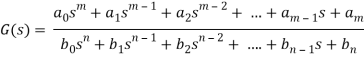
Now the equation P(s) =0 has m roots while equation Q(s) has n roots. Thus G(s) can be expressed in the factorized form as
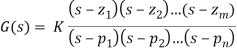
Where z1,z2…….zm are the roots of the equation P(s) =0 and P1,P2……Pn are the roots of the equation Q(s) =0.
K = a0/b0 = scale factor
Thus z1,z2…….zm,P1,P2…….Pn are the values of s and hence are complex frequencies as s variable is a complex variable.
Poles:
The values of ‘s’ that is complex frequencies which make the network function infinite when substituted in the denominator of a network are called poles of the network function.
s = p1,p2……..pn are the poles of G(s)
If such poles are real and non -repeated these are simple poles/ If a particular pole has same value twice or more than it is repeated pole. A pair of poles with complex conjugate values is called pair of complex conjugate poles.
The poles are the roots of the equation by equating denominator polynomial of the network function to zero. Such equation is called the characteristic equation of the network.
Zeros:
The value s that is complex frequencies make the network function zero when substituted in the numerator of network function called zeros of the network function.
s = z1,z2………..zm are the zeros of G(s)
The zeros are the roots of the equation by equation numerator polynomial of a system function to zero.
When the order m > n there are m-n poles at infinity while m<n then n=m is zeros at infinity. Hence for an9y rational network function poles and zeros at infinity and zero are taken into consideration in addition to finite poles and zeros . The total number of zeros is equal to the number of poles.
Example:
For the network function:
N(s) = s 2 (s+3) / (s+1) (s+2+j)(s+2-j)
At s=0 Double zero occurs and s=-3 a zero occurs
At s=-1 pole occurs
S= -2-j1 and -2 +j1 pole occurs.
N(s) = p(s)/q(s) = (ao/bo) [ (s-z1)(s-z2)………..(s-zn) / (s-p1)(s-p2)…….(s-pm)]
H=(a0/b0) is called the scale factor
Now calculating c(s), c(t) for different values of input
1) Impulse I/p
R(t) =  (t)
(t)
R(s) = 1
C(s) = R(s) wn2/s2+2 wns+wn2
C(s) = wn2/s2 +2 wn+wn2
Under this i/p (R(t) =  (t)) the output varies with different values of
  . So,
. So,
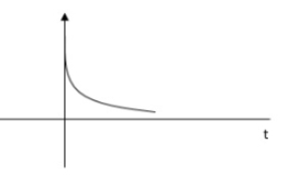
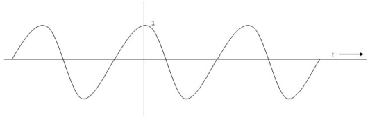
CONDITION 1: ( =0)
=0)
C(s) =wn2/s2 +wn2
Os2 +wn2 =0
S=+-jwn
C(t) = wnsinwnt
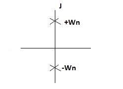
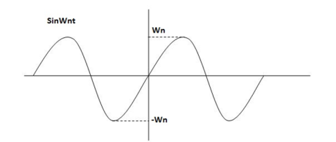
Fig. Undamped oscillations
As there in no damping i.e. oscillations at t= 0 are some at t  so, called UNDAMPED
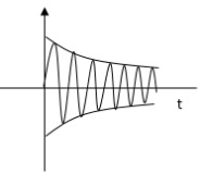
CONDITION 2: 0<<1
c(s) = R(s) wn2/s22 wn+wn2 R(t) =
  (t)
(t)
R(s) =1
C(s) = wn2/s2+2 wns+wn2
CE
S2+2 wns +wn2 =0
S2, S1 = - wn ±jwn
  1-
1- 2
2
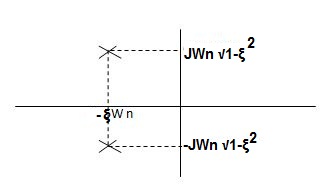
C(t) = e- wntsin( wn
 )t
)t
Wd = wn 
C(t)=e- wnt sin (wdt)
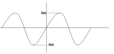
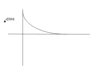
Fig. Underdamped oscillations
The oscillations are present but at t- infinity the Oscillations are 0 so, it is UNDERDAMPED
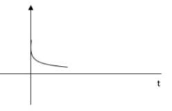
CONDITION 3 : =1
=1
C(s) = R(s) wn2/s2+2 wns+wn2
C(s)=wn2/S2 +2wns+wn2
=wn2/(s +wn)2
CE S= -Wn
C(t)= w2n/(
w2n/( )2
)2
C(t)=
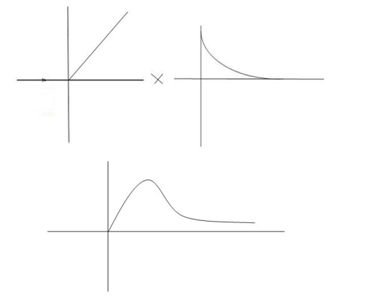
Fig. Critically damped oscillations
No damping obtained at  so is called CRITICALLY DAMPED.
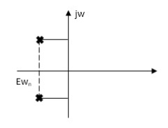
CONDITIONS 4:- >1
>1
C(s) = wn2/s22 wnS+Wn2
S1, s2 =  WN+-jwn
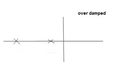
Fig. Location of poles for over damped oscillations
a) UNIT Step Input:
R(s) = 1/s
C(s)/R(s) = wn2/s2+2 wns+wn2
C(s) = R(s) wn2 /s2 +2 wns+wn2
C(s) = R(s) wn2/s2+2 wns+wn2
C(s) = R(s) wn2/s2+2 wns+wn2
C(s) = wn2s(s2+2 wns+wn2)
C(t) = 1- e wnt/
wnt/ 1-es2sin (wdt + ø)
Wd = wn 1-
1- 2
2
Ø= 
Where
Wd = Damping frequency of oscillations
Wn = natural frequency of oscillations
 wn = damping coefficient.
T= Time constant
Condition 1 = 0
= 0
C(s) = wn2 /s(s2+wn2)
C(t) = 1- e° sin wdt +ø
C(t)= 1- sin( wn +90)
C(t) = 1+cos wnt
Constant
C(t) = 1+constant

Fig. C(t) = 1+cos wnt
Condition 2: 0< <1
<1
C(s) =  /s2+
/s2+ wns +wn2
C(s) =1/s – s+ wn/s2+
 wns +wn2
=1/s – s+ wn/(s+
 wn)2+wd2-
  wn/(s+
 wn2) +wd2
Wd = wn 1-
1- 2
2
Taking Laplace inverse of above equation
L --1 s+ wn/(s+
 wn) +wd2= e-
 wnt coswdt
L-1 s+ wn/(s+
 wn)2+wd2 = e-
 wnt sinWdt
C(t) = 1-e- wnt [coswdt +
 /
/ 1-
1- 2sinwdt]
= 1-e wnt /
wnt / 1-
1- 2 sin [wdt +
  1-
1- 2/
2/ ] t>=0
C(t) = 1-e wnt/
wnt/ 1-
1- 2 sin(wdt+ø)
Ø =  1+
1+ 2/
2/
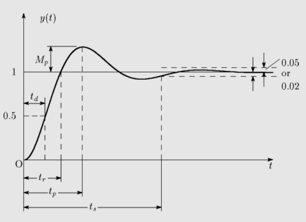
Fig. Transient Response of second order system
To find the time domain behaviour we consider a simple RLC circuit. When the poles and zeros of I(s) can be represented in terms of undamped natural frequency (wn)and damping ratio  . these can be represented as.
Wn = 1/ Lc and
  =R/2
=R/2 C/L
C/L
For RLC network the characteristics equation of any second differential equation.
s2+2 wns+wn2=0
s1s2=-2 wn+-
wn+-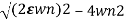 / 2
/ 2
=-2 wn+-
wn+- /2
/2
=-2 wn+-
wn+- /2
/2
=-2 wn+-2
wn+-2 / 2
/ 2
s1,s2 =- wn+-wn
So, depending an § poles can be represented in various ways
a) >1
>1
s1s2 = - wn+- wn
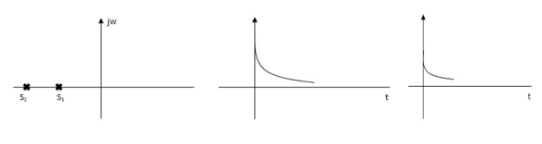
Fig. Location of Poles and system response
As s1 s2 lies on negative real axis. This corresponds to OVERDAMPED are have exponential decay from in the time domain.
b) 0< <1
<1
s1s2 = - wn+-∫wn
The poles are plotted below having both real and imaging part
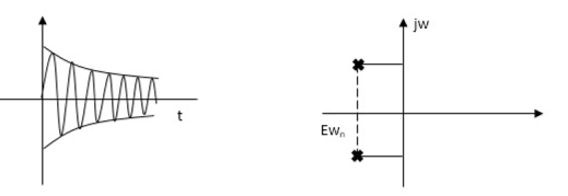
Fig. Time response Fig. Root Plot
As the roots have real and imaginary component as roots 0, this corresponds to UNDERDAMPED association. As initially oscillations exist, but oscillations seen as t-
c) =0
=0
s1s2 = - wn+- wn
s2+2 wns+w2n=0
For  =0
=0
s2+wn2=0
s=Ijwn

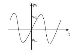
Fig. Root Plot Fig. Time response
As the complex conjugal the as at t=0 and t= same so, this is the case of UNDAMPED associations.
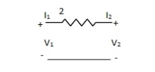
Key takeaway
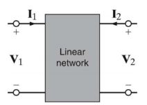
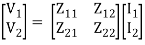
[V1] = [Z11 Z12][I1]
[V2] =[ Z21 Z22] [I2]
V1 = Z11 I1 + Z12 I2
V2 = Z21 I1 + Z22 I2
Determine Z parameters
Z11 = V1/I1 |I2 =0 open circuit input impedance
Z22 = V2/I2 |I1 =0 Open circuit output impedance
Z12 = V1/I2 | I1 =0
Z21 = V2/I1 |I2 =0
I1 = Y11 V1 + Y 12 V2
I 2 = Y21 V1 + Y 22 V2
To determine Y parameters:
y11 = I1/V1 |V2=0 ----- short circuit input admittance
y22 = I2/V2 |V1=0 ---- short circuit output admittance
y12 = I1/V2 |v1=0
y21 = I2/V1 |v2=0 trans admittance
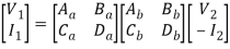
Transmission parameters
Transmission parameter [ABCD]
V1 = AV2 - BI2
I1 = CV2 - DI2
A =  I2=0
I2=0
B =  V2=0
V2=0
C =  -I2=0
-I2=0
D =  V2=0
V2=0
Symmetrical two-port N/W: -
 I2 = 0 =
  I1=0
I1=0
A = D
Reciprocal two port N/W
 I1=0 =
 I2 = 0
AD – BC = 1
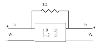
Que 1. Find all the Transmission parameters?
Solution:
-3V1 – I1 +  +
+  = 0
= 0
 +
+  = I1
= I1
 V1 – V2 = I1
 V1 = V2 + I1
V1= V2-
V2-  I1----------------(1)
I2 = 3V1 + V2 + V2 – V1
I2 = 2V1 + 2V2
2V1 = I2 - 2V2
2V1 = - 2V2 + I2
V1 = -V2 +  I2 ----------------(2)
A = -1
B = 
From (1) & (2)
-V2 +  I2 =
I2 =  I1 -
I1 -  V2
V2
 V2 - V2 +
  I2 =
I2 =  I1
I1
 I1 =
I1 =  V2 + V2 -
  I2
I2
I1 =  V2 -
V2 -  I2
I2
C = 
D = 
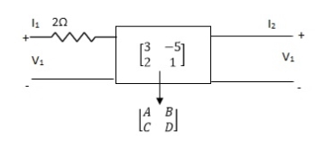
Que 2. Find all the Transmission parameters?
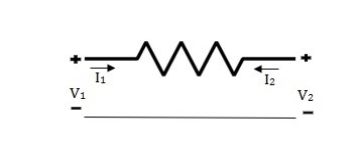
Solution: V1 = RI1 + V2 ----------------(1)
I2R = V2 – V1
I2 =  V2 -
V2 -  V1
V1
I2R = V2 – V1
V1 = I2R - V2 --------------------(2)
A = 1
B = R
From (2) in (1)
V2 - I2R = V2 + RI1
I2 = -I1
C = 0
D = 1
Que 3. Find all the Transmission parameters?
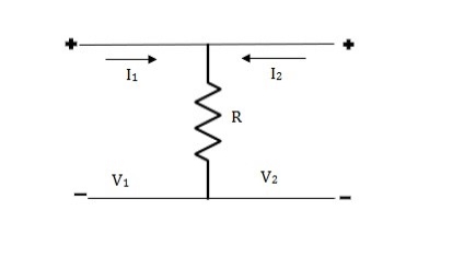
Solution: V1 = R (I1 + I2)
V2 = R (I1 + I2)
V1 = V2 + 0I2
A = 1
B = 0
V2 = RI1 + RI2
RI1= V2 - RI2
I1 =  V2 – I2
C =  , D = 1
Hybrid parameters
H-parameter: -
V1 = h11I1 + h12V2
I2 = h21I1 + h22V2
Equivalent circuit for H-parameter:
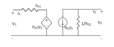
Fig. Equivalent circuit for H-parameter
h11 = |V2=0
|V2=0
h12 = I1=0
I1=0
h21 =  V2=0
V2=0
h22 =  |I1=0
|I1=0
Symmetrical two-port N/W: -
 I2 = 0 =
  |I1=0
|I1=0
∆h = 0
Reciprocal two-port N/W: -
 |I1=0 =
 |I2 = 0
h12 = h21
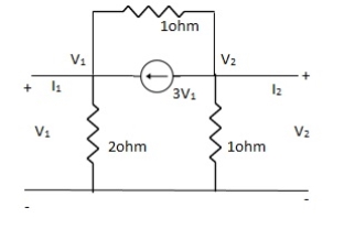
Que 4. Find all h-parameter?
Solution:  = I1
= I1
 V1 -
V1 -  = I1
= I1
 V1 =
V1 =  + I1
+ I1
V1 = +
+  I1
I1
 - + 3I1 = I2
3I1 + V2- = I2
= I2
From (1)
I2 = 3I1 + V2 –  [
[ I1 +
I1 +  V2]
V2]
I2 =  I1 +
I1 +  V2
V2
h11 = 
h12 = 
h21 = 
h22 = 
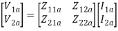
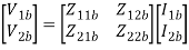
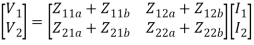
Series connection
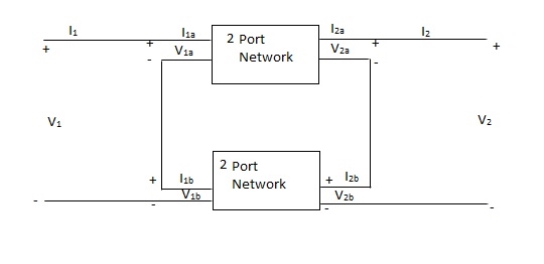
V1 = V1a +V1b
I1 = I1a = I1b
V2 = V2a +V2b
I2 = I2a = I2b
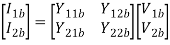
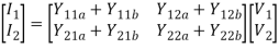
Parallel connection
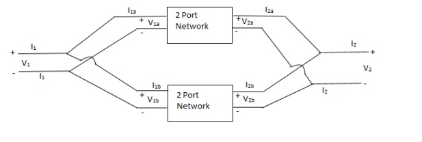
V1 = V1a = V1b

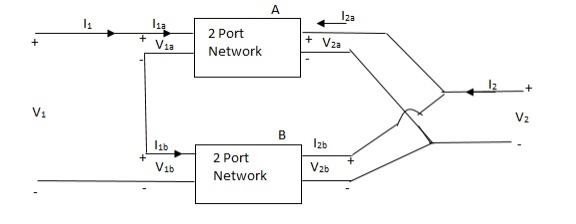
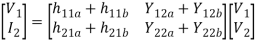
Series parallel connection
I1 = I1a = I1b
V1 = V1a +V1b
If two 2-ports are connected in series parallel then overall h-parameter is sum of individual h-parameter

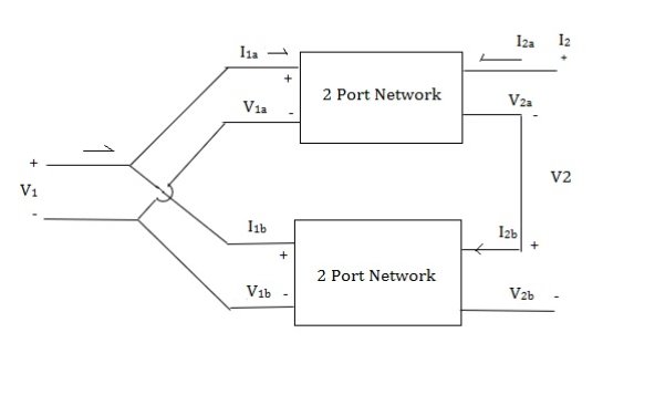
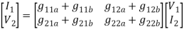
Parallel series connection
Cascade connection
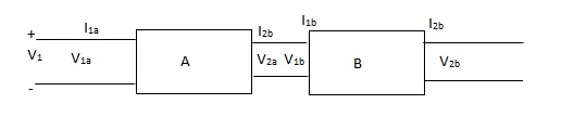
V1 = V1a, V2a = V1b, V2 = V2b
I1 = I1a, I2a = -I1b, I2 = I2b
Transmission parameter for N/W (A)

Transmission parameter for N/W (B)

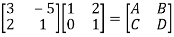
Overall transmission parameter
Que 1.
Find out overall transmission parameter?
Solution:

Que 2.
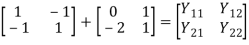
Find overall Y-parameter?
Solution:
References:
1. Mahmood Nahvi, Joseph A Edminister, “Schaum’s outline of Electric Circuits”, 6th Edition, Tata McGraw-Hill, 6th Edition, 2013
2. W. H. Hayt and J. E. Kemmerly, “Engineering Circuit Analysis”, McGraw Hill Education, 2013.
3. C. K. Alexander and M. N. O. Sadiku, “Electric Circuits”, McGraw Hill Education, 2004.
4. K. V. V. Murthy and M. S. Kamath, “Basic Circuit Analysis”, Jaico Publishers, 1999.
5. K. Sureshkumar, “Electric Circuits & Network”, Pearson Publication
6. Del Toro, “Electrical circuit”, Prentice Hall


