Unit - 3
Convolution
Using the linear property of the system the interchange operator T with the summation k to obtain
y(n) =[ T δ(n-k)] ----------------------------------------------(4)
The response to the shifted impulses is represented as h(n,k)
h(n,k) = T[ δ(n-k)]
Now
y(n) = h(n,k) -----------------------------------------------------------(5)
For time-invariant system
h(n,k) =h(n-k) ----------------------------------------------------------------------(6)
Substituting (6) in (5) we get
y(n) = h(n-k) ------------------------------------------------------------------(7)
Thus, the output of the LTI system is given by the weighted sum of time-shifted responses.
The sum in eq(7) is termed as convolution sum which is given by
y(n) = x(n) * h(n) -----------------------------------------------------------------------------(8)
* denotes convolution operation.
Problem:
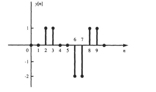
The impulse response h[n] of a discrete-time LTI system. Determine and sketch the output y[n] of this system to the input x[n]

h[n] = δ[n] + δ[n-1] + δ[n-2]+δ[n-3]+δ[n-4]+δ[n-5]
x[n] = δ[n-2] - δ[n-4]
x[n] * h[n] = x[n] * { δ[n] + δ[n-1] + δ[n-2]+δ[n-3]+δ[n-4]+δ[n-5]}
= x[n] + x[n-1] + x[n-2]+ x[n-3]+ x[n-4]+ x[n-5]
y[n] =δ[n-2]-δ[n-4]+δ[n-3]-δ[n-5] +δ[n-4]-δ[n-6]+δ[n-5]-δ[n-7] - δ[n-6]+δ[n-8]-δ[n-7]+δ[n-9]}
= δ[n-2]+δ[n-3]-2δ[n-6]-2δ[n-7] + δ[n-8]+δ[n-9]
y[n] = {0,0,1,1,0,0,-2,-2,1,1}

Computation of convolution sum
For x(n) = {3,2,-1,2,4,1} find the sum of the shifted unit impulses.
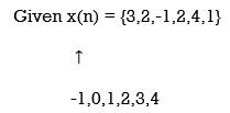
x(-1) = 3. x(0)=2 , x(1)=-1, x(2) =2, x(3)=4,x(4) =1
x(n) =  δ(n-k)
x(-1) δ(n+1) + x(0) δ(n) + x(1) δ(n-1) + x(2) δ(n-2)+ x(3) δ(n-3)+ x(4) δ(n-4)
We get
3 δ(n+1) + 2 δ(n) - δ(n-1) + 2 δ(n-2)+ 4 δ(n-3)+ δ(n-4)
Properties of Convolution Sum
Commutative Property
The commutative property states that the order in which two sequences are convolved is not important. Mathematically, the commutative property is
x(n) * h(n) = h(n) * x(n)
From a systems point of view, this property states that a system with a unit sample response h(n) and input x(n) behaves in the same way as a system with unit sample response x(n) and an input h(n).
This is illustrated in Fig. (a).
Associative Property
The convolution operator satisfies the associative property, which is
[x(n) * h1(n) } * h2(n) = x(n) * { h1(n) * h2(n)}
From a systems point of view, the associative property states that if two systems with unit sample responses h1(n) and h2(n) are connected in cascade as shown in Fig. (b), an equivalent system is one that has a unit sample response equal to the convolution of h1 (n) and h2(n):
Heq = h1(n) * h2(n)

Figure 1. Commutative, Associative, and Distributive Property.
Distributive Property
The distributive property of the convolution operator states that
x(n) * {hl(n) + h2(n)} = x(n) * hJ(n) + x(n) * h2(n)
From a systems point of view, this property asserts that if two systems with unit sample responses h J (n) and h2(n) are connected in parallel, as illustrated in Fig. (c), an equivalent system is one that has a unit sample response equal to the sum of hJ(n) and h2(n):
Heq (n) = h1(n) + h2(n)
Consider an LTI system that is initially related at t=0. If the input of the system is an impulse, then the output of the system is denoted by h(t) is called the impulse response of the system.
We can denote
h(t) = T [ δ(t)]
We know that any arbitrary signal x(t) can be represented as
x(t) =  ( t-
( t- d
d ------------------------------------------------------(1)
The system output is given by
y(t) = T[x(t)] --------------------------------------------------------------------------------(2)
Substituting (1) in (2)
y(t) = T [  ( t-
( t- d
d --------------------------------------------------------(3)
For linear system
y(t) =[  T[
T[ ( t-
( t- d
d --------------------------------------------(4)
If the response of the system due to impulse δ(t) is h(t) then the response of the system due to delayed impulse is
h(t, = T [ δ(t-T)] --------------------------------------------------------------(5)
Substituting (5) in (4) we get
y(t) =[  h(t,τ) dτ-------------------------------------------------------(6)
For a time-invariant system the output due to the delayed input by T is equal to delayed output by T, That is
h(t,τ) = h(t-τ) ---------------------------------------------------------------(7)
Substituting (7) in (6) we get
y(t) = h(t-τ) dτ -----------------------------------------------------------(8)
This is called convolution Integral.The convolution of two signal x(t) and h(t) can be represented as
y(t) = x(t) * h(t)
Computation of convolution integral using the graphical method
The procedure is as follows:
- For the given signals x(t) and h(t) graph the signals x(τ) and h(τ) as a function of independent variable τ.
- Obtain the signal h(t-τ) by folding h(τ) about τ=0 and then time-shifting by time t.
- Graph both signals x(τ) and h(t-τ) on the same τ-axis beginning with very large negative time shift t.
- Multiply the two signals x(τ) h(t-τ) and integrate over the overlapping interval oftwo signals to obtain y(t)
- Increase the time shift and take the new interval whenever the function of either x(τ) and h(t-τ) changes. The value of t at which the change occurs defines the end of the current interval and the beginning of a new interval. Calculate y(t) using step 4.
- Repeat steps 5 and 4 for all intervals.
Unit step to rectangular:
Find the convolution of x(t) and h(t)
x(t) =10 
= 0 otherwise

Fig 2. x(t) and h(t)

Figure 3: x(τ) and h(t-τ)
As shown in Figure the signals x(τ) and h(t-τ) does not overlap for t<0. Therefore the product x(τ) h(t-τ) is zero.
That is,
y(t) =  h(t-τ) =0for t<0
Now the shift the signal h(t-τ) right until the right edge of the signal h(t-τ) intersects the left edge of x(τ).
In the interval 0 
y(t) =  = t
= t
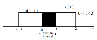
Figure 4. Product of x(t) and h(t-τ)
In the interval 2
y(t) =  = 2
= 2
In the interval 3 

Figure 5. Product of h(t-τ) x(τ)
y(t) = = 2 – (t-3)
= 5-t.
For t

Figure 6. Product of x(τ) h(t-τ) for t 5
5
The signals x(τ) and h(t-τ) do not overlap. Therefore y(t)=0.
y(t) = 0 for t<0
=t for 1 
= 2 for2 
= 5-t for 3 
=0 for t  5.
5.
The sketch y(t) is as shown in figure

Figure 7. The output waveform
Unit Step to Exponential
Given:
x(t) = e -2 u(t)h(t) = u(t+2)

Figure 8. x(t) and h(t)

Figure 9. Product exponential signal and unit step signal
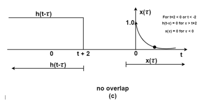
Figure 10. Product of exponential signal and delayed unit step signal

Figure 11. The output waveform
Figure (a) shows x(t) and h(t). Fig (b) shows x(τ) and h(-τ) as functions of τ. The function h(-τ) can be obtained by folding the signal h(τ) about τ=0.
Figure (c ) shows that signal h(t-τ) is sketched for t<-2 by shifting h(τ) to left. For t<-2 x(τ) and h(t-τ) does not overlap and the product x(τ) h(t-τ) =0 that is
y(t) =0 for t<-2
Now increase the time shift until the signal h(t-τ) intersects x(τ). Figure (d) shows the situation for t>-2.
Here x(τ) =0 forτ<0and h(t-τ) does not overlap and the product x(τ) h(t-τ) =0 that is
y(t)=0for t<-2
Now increase the time shift t until the signal h(t-τ) intersects x(τ).
Figure (d) shows the situation for t>-2. Here x(τ) and h(t-τ) overlapped. But x(τ) =0 for τ<0 and h(t-τ) = 0 for τ> t+2. Therefore, the integration interval is from τ=0 to τ=t+2
y(t) =  h(t-τ) dτ
=  -2τdτ
-2τdτ
= -1/2e -2 τ|0t+2
= -1/2 [ e -2 (t+2) -1]
= 1 – e -2(t+2)/2
y(t) = 0 for t<-2
= 1 – e-2(t+2)/2 for t  -2
-2
Exponential to exponential
x(t) = e -|t|
h(t) = e -2(t+1) u(t+1)

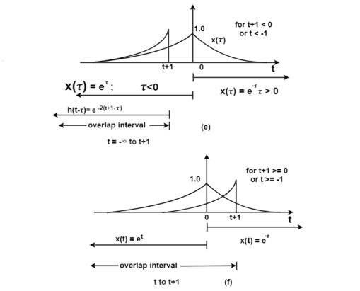
Figure 12. Steps for exponential-to-exponential convolution
Fig (a) shows the signal x(t). In fig(b) the signal e -2t u(t) is sketched from which can be obtained from the signal h(t) = e -2(t+1) u(t+1)
Fig ( c ) shows the signal h(-τ) which can be obtained by folding the signal h(τ) about t=0.
In fig (e )the signals x(τ) and h(t-τ) are drawn on the same axis.
For (t+1) <0or t<-1 the signals x(τ) and h(t-τ) overlap over the interval - τ
τ t+1.
t+1.
During this interval the signal x(τ) = e τ and h(t-τ) = e -2 (t+1-τ). Therefore, for
t<-1
y(t) =  τe -2(t+1-τ)dτ
= e -2t -2 3 τdτ
3 τdτ
= e -2(t+1) /3e 3 τ |-  0+ e -2 (t+1) e τ| 0t+1
= e -2(t+1) /3 [1] + e –2(t+1) [ e t+1 -1 ]
= e -2(t+1) /3 + e –(t+1) – e -2 (t+1)
= e –(t+1) – 2/3 e -2(t+1)
y (t) = 1/3 e t+1for t<-1
= e –(t+1) – 2/3 e -2(t+1) for t  -1
-1
Rectangular to rectangular
Find the response of the system y(t) of an LTI system whose x(t) and h(t) are as shown in the figure.

Fig 13. x(t) and h(t) signals
The figure shows the signal x(τ) and h(-τ). In the figure, the signals x(τ) and h(t-τ) do not overlap. Therefore, the product x(τ) h(t-τ) is equal to zero. For t<-2 the signals x(τ) and h(t-τ) does not overlap. Therefore, the product x(τ) h(t-τ) is equal to zero.
Hence
y(t) =  h(t-τ) dτ
= 0 for t<-2

Fig 14. Convolution of x(t) and h(-τ)
Now increase the value of t and shift the signal h(t-τ) as shown in figure. Here the overlap interval is τ = 0 to t+2 . In this interval x(τ) = 1.0 ; h(t-τ) = 2.0

Figure 15. Convolution of x(τ) h(t-τ)
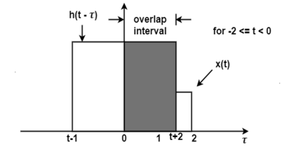
Figure 16. Output of the convolution x(t) and h(t)
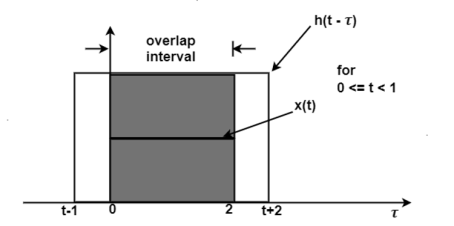
Figure 17. Output for t<1
Therefore,
y(t) =  d τ
d τ
= 2τ | 0t+2= 2(t+2) = 2t + 4
This value holds for -2
In the interval 0  1 the overlap interval is constant that is from τ=0to τ=2
Therefore
y(t) =  d τ=2 τ | 02 =4

Figure 18. Output waveform for t<3
If we shift h(t-τ) further the resultant diagram is shown in fig 4.29. Here the overlap interval is from τ = t-1 to τ=2. Therefore, for the interval 1 
y(t) =  dτ
dτ
= 2τ | 2t-1
= 2[ 2 – (t-1)]
= 6 – 2t
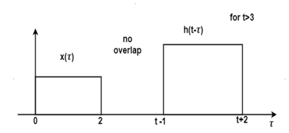
Figure 19. Output waveform for t>3
For t>3 the signals do not overlap. Therefore
y(t) = 0 for t>3
y(t) = 0 for t  -2
-2
= 2t + 4for -2  <0
<0
= 4for 0  t <1
t <1
= 6 -2t for 1  <3
<3
=0for t 
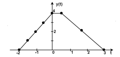
Figure 20. Final output waveform
Unit step to unit step
x(t) = u(t+1)h(t) = u(t-2)
The signals x(t) and h(t) are shown in figure.

Figure 21. Unit step signal x(t)

Figure 22. Unit step signal
The figure below the signals x(τ) and h(t-τ) on the same axis. Thesignal h(t-τ) is obtained by folding the signal h(τ) about τ=0 and then left shiftingh(-τ).
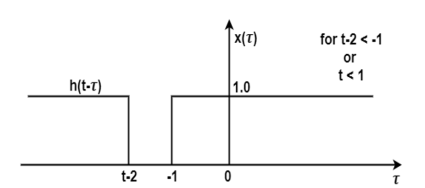
Figure 23. Convolution of x(τ) and folding signal h(t-τ)
For t<1 the overlap area of x(τ)and h(t-τ) is zero. Therefore y(t) =0. Now shift the signal h(t-τ) right as shown in the figure.

Figure 24. Convolution for t>1
Here the signal x(τ)and h(t-τ) do overlap over the interval -1 < t-2 . Therefore
y(t) =  h(t-τ) d τ
 = τ | -1-2 = (t-2) – (-1) = t-1
= y(t) =0 for t<1
= t-1 for t 1
1
The signal y(t) is sketched as shown in figure.
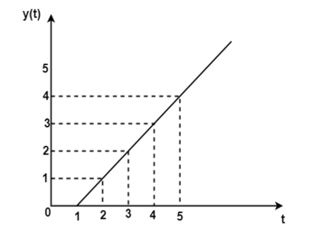
Figure 25. The output waveform
The Linear time invariant (LTI) system:
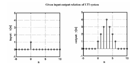
Systems which satisfy the condition of linearity as well as time invariance are known as linear time invariant systems. Throughout the rest of the course we shall be dealing with LTI systems. If the output of the system is known for a particular input, it is possible to obtain the input for a number of other inputs. We shall see through examples, the procedure to compute the output from a given input-output relation, for LTI systems.
Example – 1:
Convolution:
A continuous time system as shown below, accepts a continuous time signal x(t) and gives out a transformed continuous time signal y(t).
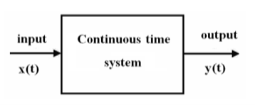
Figure 26. The continuous time system
Some of the different methods of representing the continuous time systems are:
i) Differential equation
Ii) Block diagram
Iii) Impulse response
Iv) Frequency response
v) Laplace-transform
Convolution Sum:
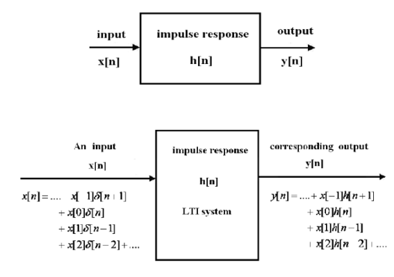
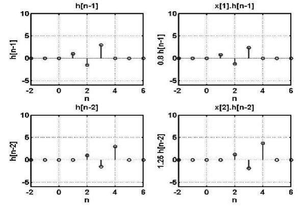
We now attempt to obtain the output of a digital system for an arbitrary input x[n], from the knowledge of the system impulse response h[n].
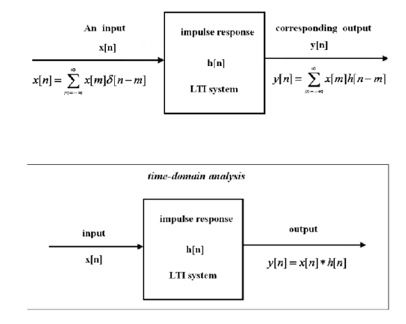
y[n] = x[n] * h[n]
Methods of evaluating the convolution sum:
Given the system impulse response h[n], and the input x[n], the system output y[n], is given by the convolution sum:
y[n] = 
Problem:
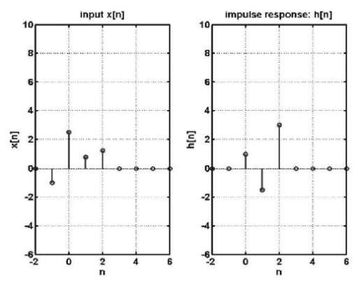
To obtain the digital system output y[n], given the system impulse response h[n], and the system input x[n] as:
h[n] = [ 1, -1.5, 3]


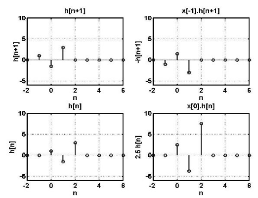

Convolution as matrix multiplication:
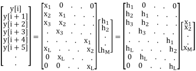
Given
x[n] = [x1 x2 ... xL] starting from Nx
And
h[n] = [h1 h2 ... hM] starting from NH
Step 1: Length of convoluted sequence is NUM = (L+M-1)
Step 2: The convoluted sequence starts at i = Nx + NH
Step 3: The convolution is given by the following matrix multiplication

The dimension of the above matrices are:
[NUM by 1] = [NUM by M][M by 1] = [NUM by L][L by 1]
For the given example:
x[n] is length L=4, and starts at Nx = -1
h[n] is of length M=3 and starts at NH = 0
Step 1: Length of convoluted sequence is NUM = (L+M-1)=6
Step 2: The convoluted sequence starts at i = (-1+0) = (-1)


Linear constant coefficient differential equation:
The continuous time linear time invariant (LTI) systems are described by their linear constant coefficient differential equations. For this, let us consider a first order differential equation as under 
Where x(t) and y(t) are the input and output of the continuous time LTI system. A is a constant value. The first order differential equation can be extended for higher order differential equations. A general Nth order linear constant coefficient differential equation can be given by

The complete solution of differential equation consists of the sum of particular solution yp(t) and homogenous solution yn(t).
The homogeneous solution of a differential equation is possible by substituting

This solution to differential equation is also known as natural response of the system.
A particular case of differential equation is determined by putting N=0, we obtain

Transfer function:
Transfer functions are commonly used in the analysis of systems such as single-input single-output filters, typically within the fields of signal processing, communication theory, and control theory. The term is often used exclusively to refer to linear, time-invariant systems (LTI). Most real systems have non-linear input/output characteristics, but many systems, when operated within nominal parameters have behaviour that is close enough to linear that LTI system theory is an acceptable representation of the input/output behaviour.
The descriptions below are given in terms of a complex variables, s = σ + j. ω, which bears a brief explanation. In many applications, it is sufficient to define σ = 0 ( and s = j.ω), which reduces the Laplace transforms with complex arguments to Fourier transforms with real argument ω. The applications where this is common are ones where there is interest only in the steady-state response of an LTI system, not the fleeting turn-on and turn-off behaviours or stability issues. That is usually, the case for signal processing and communication theory.
Thus, for continuous-time input signal x(t) and output y(t0), the transfer function H(s) is the linear mapping of the Laplace transform of the input, X(s) – L[x(t)], to the Laplace transform of the output Y(s) = L[y(t)]:
Y(s) = H(s) X(s)


References:
1. Signals and Systems by Simon Haykin
2. Signals and Systems by Ganesh Rao
3. R.F. Ziemer, W.H Tranter and J.D.R.Fannin, “Signals and Systems - Continuous and Discrete”, Forth Edition Prentice Hall.
4. M. J. Roberts, “Signals and Systems”, 2003, Tata McGraw-Hill
Unit - 3
Convolution
Using the linear property of the system the interchange operator T with the summation k to obtain
y(n) =[ T δ(n-k)] ----------------------------------------------(4)
The response to the shifted impulses is represented as h(n,k)
h(n,k) = T[ δ(n-k)]
Now
y(n) = h(n,k) -----------------------------------------------------------(5)
For time-invariant system
h(n,k) =h(n-k) ----------------------------------------------------------------------(6)
Substituting (6) in (5) we get
y(n) = h(n-k) ------------------------------------------------------------------(7)
Thus, the output of the LTI system is given by the weighted sum of time-shifted responses.
The sum in eq(7) is termed as convolution sum which is given by
y(n) = x(n) * h(n) -----------------------------------------------------------------------------(8)
* denotes convolution operation.
Problem:
The impulse response h[n] of a discrete-time LTI system. Determine and sketch the output y[n] of this system to the input x[n]

h[n] = δ[n] + δ[n-1] + δ[n-2]+δ[n-3]+δ[n-4]+δ[n-5]
x[n] = δ[n-2] - δ[n-4]
x[n] * h[n] = x[n] * { δ[n] + δ[n-1] + δ[n-2]+δ[n-3]+δ[n-4]+δ[n-5]}
= x[n] + x[n-1] + x[n-2]+ x[n-3]+ x[n-4]+ x[n-5]
y[n] =δ[n-2]-δ[n-4]+δ[n-3]-δ[n-5] +δ[n-4]-δ[n-6]+δ[n-5]-δ[n-7] - δ[n-6]+δ[n-8]-δ[n-7]+δ[n-9]}
= δ[n-2]+δ[n-3]-2δ[n-6]-2δ[n-7] + δ[n-8]+δ[n-9]
y[n] = {0,0,1,1,0,0,-2,-2,1,1}
Computation of convolution sum
For x(n) = {3,2,-1,2,4,1} find the sum of the shifted unit impulses.

x(-1) = 3. x(0)=2 , x(1)=-1, x(2) =2, x(3)=4,x(4) =1
x(n) =  δ(n-k)
x(-1) δ(n+1) + x(0) δ(n) + x(1) δ(n-1) + x(2) δ(n-2)+ x(3) δ(n-3)+ x(4) δ(n-4)
We get
3 δ(n+1) + 2 δ(n) - δ(n-1) + 2 δ(n-2)+ 4 δ(n-3)+ δ(n-4)
Properties of Convolution Sum
Commutative Property
The commutative property states that the order in which two sequences are convolved is not important. Mathematically, the commutative property is
x(n) * h(n) = h(n) * x(n)
From a systems point of view, this property states that a system with a unit sample response h(n) and input x(n) behaves in the same way as a system with unit sample response x(n) and an input h(n).
This is illustrated in Fig. (a).
Associative Property
The convolution operator satisfies the associative property, which is
[x(n) * h1(n) } * h2(n) = x(n) * { h1(n) * h2(n)}
From a systems point of view, the associative property states that if two systems with unit sample responses h1(n) and h2(n) are connected in cascade as shown in Fig. (b), an equivalent system is one that has a unit sample response equal to the convolution of h1 (n) and h2(n):
Heq = h1(n) * h2(n)
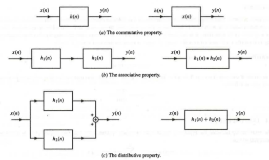
Figure 1. Commutative, Associative, and Distributive Property.
Distributive Property
The distributive property of the convolution operator states that
x(n) * {hl(n) + h2(n)} = x(n) * hJ(n) + x(n) * h2(n)
From a systems point of view, this property asserts that if two systems with unit sample responses h J (n) and h2(n) are connected in parallel, as illustrated in Fig. (c), an equivalent system is one that has a unit sample response equal to the sum of hJ(n) and h2(n):
Heq (n) = h1(n) + h2(n)
Consider an LTI system that is initially related at t=0. If the input of the system is an impulse, then the output of the system is denoted by h(t) is called the impulse response of the system.
We can denote
h(t) = T [ δ(t)]
We know that any arbitrary signal x(t) can be represented as
x(t) =  ( t-
( t- d
d ------------------------------------------------------(1)
The system output is given by
y(t) = T[x(t)] --------------------------------------------------------------------------------(2)
Substituting (1) in (2)
y(t) = T [  ( t-
( t- d
d --------------------------------------------------------(3)
For linear system
y(t) =[  T[
T[ ( t-
( t- d
d --------------------------------------------(4)
If the response of the system due to impulse δ(t) is h(t) then the response of the system due to delayed impulse is
h(t, = T [ δ(t-T)] --------------------------------------------------------------(5)
Substituting (5) in (4) we get
y(t) =[  h(t,τ) dτ-------------------------------------------------------(6)
For a time-invariant system the output due to the delayed input by T is equal to delayed output by T, That is
h(t,τ) = h(t-τ) ---------------------------------------------------------------(7)
Substituting (7) in (6) we get
y(t) = h(t-τ) dτ -----------------------------------------------------------(8)
This is called convolution Integral.The convolution of two signal x(t) and h(t) can be represented as
y(t) = x(t) * h(t)
Computation of convolution integral using the graphical method
The procedure is as follows:
- For the given signals x(t) and h(t) graph the signals x(τ) and h(τ) as a function of independent variable τ.
- Obtain the signal h(t-τ) by folding h(τ) about τ=0 and then time-shifting by time t.
- Graph both signals x(τ) and h(t-τ) on the same τ-axis beginning with very large negative time shift t.
- Multiply the two signals x(τ) h(t-τ) and integrate over the overlapping interval oftwo signals to obtain y(t)
- Increase the time shift and take the new interval whenever the function of either x(τ) and h(t-τ) changes. The value of t at which the change occurs defines the end of the current interval and the beginning of a new interval. Calculate y(t) using step 4.
- Repeat steps 5 and 4 for all intervals.
Unit step to rectangular:
Find the convolution of x(t) and h(t)
x(t) =10 
= 0 otherwise

Fig 2. x(t) and h(t)

Figure 3: x(τ) and h(t-τ)
As shown in Figure the signals x(τ) and h(t-τ) does not overlap for t<0. Therefore the product x(τ) h(t-τ) is zero.
That is,
y(t) =  h(t-τ) =0for t<0
Now the shift the signal h(t-τ) right until the right edge of the signal h(t-τ) intersects the left edge of x(τ).
In the interval 0 
y(t) =  = t
= t

Figure 4. Product of x(t) and h(t-τ)
In the interval 2
y(t) =  = 2
= 2
In the interval 3 
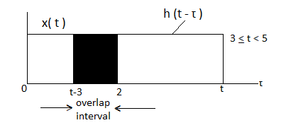
Figure 5. Product of h(t-τ) x(τ)
y(t) = = 2 – (t-3)
= 5-t.
For t

Figure 6. Product of x(τ) h(t-τ) for t 5
5
The signals x(τ) and h(t-τ) do not overlap. Therefore y(t)=0.
y(t) = 0 for t<0
=t for 1 
= 2 for2 
= 5-t for 3 
=0 for t  5.
5.
The sketch y(t) is as shown in figure

Figure 7. The output waveform
Unit Step to Exponential
Given:
x(t) = e -2 u(t)h(t) = u(t+2)

Figure 8. x(t) and h(t)

Figure 9. Product exponential signal and unit step signal

Figure 10. Product of exponential signal and delayed unit step signal
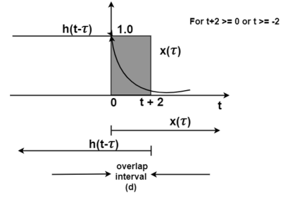
Figure 11. The output waveform
Figure (a) shows x(t) and h(t). Fig (b) shows x(τ) and h(-τ) as functions of τ. The function h(-τ) can be obtained by folding the signal h(τ) about τ=0.
Figure (c ) shows that signal h(t-τ) is sketched for t<-2 by shifting h(τ) to left. For t<-2 x(τ) and h(t-τ) does not overlap and the product x(τ) h(t-τ) =0 that is
y(t) =0 for t<-2
Now increase the time shift until the signal h(t-τ) intersects x(τ). Figure (d) shows the situation for t>-2.
Here x(τ) =0 forτ<0and h(t-τ) does not overlap and the product x(τ) h(t-τ) =0 that is
y(t)=0for t<-2
Now increase the time shift t until the signal h(t-τ) intersects x(τ).
Figure (d) shows the situation for t>-2. Here x(τ) and h(t-τ) overlapped. But x(τ) =0 for τ<0 and h(t-τ) = 0 for τ> t+2. Therefore, the integration interval is from τ=0 to τ=t+2
y(t) =  h(t-τ) dτ
=  -2τdτ
-2τdτ
= -1/2e -2 τ|0t+2
= -1/2 [ e -2 (t+2) -1]
= 1 – e -2(t+2)/2
y(t) = 0 for t<-2
= 1 – e-2(t+2)/2 for t  -2
-2
Exponential to exponential
x(t) = e -|t|
h(t) = e -2(t+1) u(t+1)
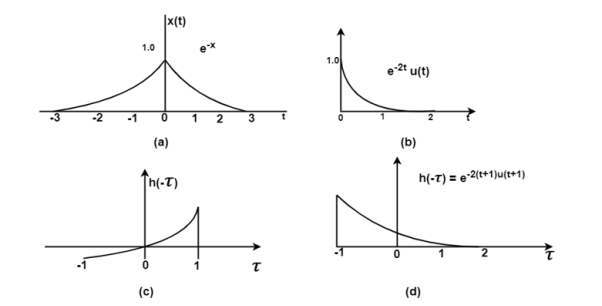

Figure 12. Steps for exponential-to-exponential convolution
Fig (a) shows the signal x(t). In fig(b) the signal e -2t u(t) is sketched from which can be obtained from the signal h(t) = e -2(t+1) u(t+1)
Fig ( c ) shows the signal h(-τ) which can be obtained by folding the signal h(τ) about t=0.
In fig (e )the signals x(τ) and h(t-τ) are drawn on the same axis.
For (t+1) <0or t<-1 the signals x(τ) and h(t-τ) overlap over the interval - τ
τ t+1.
t+1.
During this interval the signal x(τ) = e τ and h(t-τ) = e -2 (t+1-τ). Therefore, for
t<-1
y(t) =  τe -2(t+1-τ)dτ
= e -2t -2 3 τdτ
3 τdτ
= e -2(t+1) /3e 3 τ |-  0+ e -2 (t+1) e τ| 0t+1
= e -2(t+1) /3 [1] + e –2(t+1) [ e t+1 -1 ]
= e -2(t+1) /3 + e –(t+1) – e -2 (t+1)
= e –(t+1) – 2/3 e -2(t+1)
y (t) = 1/3 e t+1for t<-1
= e –(t+1) – 2/3 e -2(t+1) for t  -1
-1
Rectangular to rectangular
Find the response of the system y(t) of an LTI system whose x(t) and h(t) are as shown in the figure.
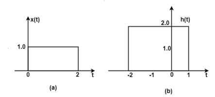
Fig 13. x(t) and h(t) signals
The figure shows the signal x(τ) and h(-τ). In the figure, the signals x(τ) and h(t-τ) do not overlap. Therefore, the product x(τ) h(t-τ) is equal to zero. For t<-2 the signals x(τ) and h(t-τ) does not overlap. Therefore, the product x(τ) h(t-τ) is equal to zero.
Hence
y(t) =  h(t-τ) dτ
= 0 for t<-2
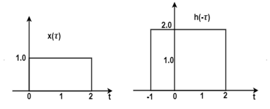
Fig 14. Convolution of x(t) and h(-τ)
Now increase the value of t and shift the signal h(t-τ) as shown in figure. Here the overlap interval is τ = 0 to t+2 . In this interval x(τ) = 1.0 ; h(t-τ) = 2.0
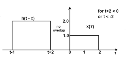
Figure 15. Convolution of x(τ) h(t-τ)

Figure 16. Output of the convolution x(t) and h(t)

Figure 17. Output for t<1
Therefore,
y(t) =  d τ
d τ
= 2τ | 0t+2= 2(t+2) = 2t + 4
This value holds for -2
In the interval 0  1 the overlap interval is constant that is from τ=0to τ=2
Therefore
y(t) =  d τ=2 τ | 02 =4
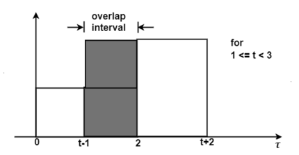
Figure 18. Output waveform for t<3
If we shift h(t-τ) further the resultant diagram is shown in fig 4.29. Here the overlap interval is from τ = t-1 to τ=2. Therefore, for the interval 1 
y(t) =  dτ
dτ
= 2τ | 2t-1
= 2[ 2 – (t-1)]
= 6 – 2t

Figure 19. Output waveform for t>3
For t>3 the signals do not overlap. Therefore
y(t) = 0 for t>3
y(t) = 0 for t  -2
-2
= 2t + 4for -2  <0
<0
= 4for 0  t <1
t <1
= 6 -2t for 1  <3
<3
=0for t 

Figure 20. Final output waveform
Unit step to unit step
x(t) = u(t+1)h(t) = u(t-2)
The signals x(t) and h(t) are shown in figure.

Figure 21. Unit step signal x(t)
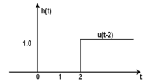
Figure 22. Unit step signal
The figure below the signals x(τ) and h(t-τ) on the same axis. Thesignal h(t-τ) is obtained by folding the signal h(τ) about τ=0 and then left shiftingh(-τ).

Figure 23. Convolution of x(τ) and folding signal h(t-τ)
For t<1 the overlap area of x(τ)and h(t-τ) is zero. Therefore y(t) =0. Now shift the signal h(t-τ) right as shown in the figure.
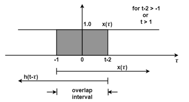
Figure 24. Convolution for t>1
Here the signal x(τ)and h(t-τ) do overlap over the interval -1 < t-2 . Therefore
y(t) =  h(t-τ) d τ
 = τ | -1-2 = (t-2) – (-1) = t-1
= y(t) =0 for t<1
= t-1 for t 1
1
The signal y(t) is sketched as shown in figure.

Figure 25. The output waveform
The Linear time invariant (LTI) system:
Systems which satisfy the condition of linearity as well as time invariance are known as linear time invariant systems. Throughout the rest of the course we shall be dealing with LTI systems. If the output of the system is known for a particular input, it is possible to obtain the input for a number of other inputs. We shall see through examples, the procedure to compute the output from a given input-output relation, for LTI systems.
Example – 1:

Convolution:
A continuous time system as shown below, accepts a continuous time signal x(t) and gives out a transformed continuous time signal y(t).

Figure 26. The continuous time system
Some of the different methods of representing the continuous time systems are:
i) Differential equation
Ii) Block diagram
Iii) Impulse response
Iv) Frequency response
v) Laplace-transform
Convolution Sum:
We now attempt to obtain the output of a digital system for an arbitrary input x[n], from the knowledge of the system impulse response h[n].


y[n] = x[n] * h[n]
Methods of evaluating the convolution sum:
Given the system impulse response h[n], and the input x[n], the system output y[n], is given by the convolution sum:
y[n] = 
Problem:
To obtain the digital system output y[n], given the system impulse response h[n], and the system input x[n] as:
h[n] = [ 1, -1.5, 3]


Convolution as matrix multiplication:
Given
x[n] = [x1 x2 ... xL] starting from Nx
And
h[n] = [h1 h2 ... hM] starting from NH
Step 1: Length of convoluted sequence is NUM = (L+M-1)
Step 2: The convoluted sequence starts at i = Nx + NH
Step 3: The convolution is given by the following matrix multiplication
The dimension of the above matrices are:
[NUM by 1] = [NUM by M][M by 1] = [NUM by L][L by 1]
For the given example:
x[n] is length L=4, and starts at Nx = -1
h[n] is of length M=3 and starts at NH = 0
Step 1: Length of convoluted sequence is NUM = (L+M-1)=6
Step 2: The convoluted sequence starts at i = (-1+0) = (-1)


Linear constant coefficient differential equation:
The continuous time linear time invariant (LTI) systems are described by their linear constant coefficient differential equations. For this, let us consider a first order differential equation as under 
Where x(t) and y(t) are the input and output of the continuous time LTI system. A is a constant value. The first order differential equation can be extended for higher order differential equations. A general Nth order linear constant coefficient differential equation can be given by

The complete solution of differential equation consists of the sum of particular solution yp(t) and homogenous solution yn(t).
The homogeneous solution of a differential equation is possible by substituting

This solution to differential equation is also known as natural response of the system.
A particular case of differential equation is determined by putting N=0, we obtain

Transfer function:
Transfer functions are commonly used in the analysis of systems such as single-input single-output filters, typically within the fields of signal processing, communication theory, and control theory. The term is often used exclusively to refer to linear, time-invariant systems (LTI). Most real systems have non-linear input/output characteristics, but many systems, when operated within nominal parameters have behaviour that is close enough to linear that LTI system theory is an acceptable representation of the input/output behaviour.
The descriptions below are given in terms of a complex variables, s = σ + j. ω, which bears a brief explanation. In many applications, it is sufficient to define σ = 0 ( and s = j.ω), which reduces the Laplace transforms with complex arguments to Fourier transforms with real argument ω. The applications where this is common are ones where there is interest only in the steady-state response of an LTI system, not the fleeting turn-on and turn-off behaviours or stability issues. That is usually, the case for signal processing and communication theory.
Thus, for continuous-time input signal x(t) and output y(t0), the transfer function H(s) is the linear mapping of the Laplace transform of the input, X(s) – L[x(t)], to the Laplace transform of the output Y(s) = L[y(t)]:
Y(s) = H(s) X(s)


References:
1. Signals and Systems by Simon Haykin
2. Signals and Systems by Ganesh Rao
3. R.F. Ziemer, W.H Tranter and J.D.R.Fannin, “Signals and Systems - Continuous and Discrete”, Forth Edition Prentice Hall.
4. M. J. Roberts, “Signals and Systems”, 2003, Tata McGraw-Hill