Unit - 6
State variable methods of analysis
The state of a system is a minimal set of variables known as state variables. The knowledge of these variables at any instance of time together with the knowledge of the inputs for the same instance of time determines the complete behaviour of the system. The fewer drawbacks in the transfer function method for representing any system led to the use of state variables in the analysis of the system. Few advantages are listed below:
- The state-space can be used for linear or nonlinear, time-variant, or time-invariant systems.
- It is easier to apply where Laplace transform cannot be applied.
- The nth order differential equation can be expressed as the 'n' equation of the first order.
- It is a time-domain method.
- As this is a time-domain method, therefore this method is suitable for digital computer computation.
- Based on the given performance index, this system can be designed for optimal conditions.
Representation of state-space: The system shown below has ‘m’ inputs, ‘p, outputs, and ‘n’ number of state variables. The state equation gives us the relation between the state variables and the inputs.

Fig 1 State variable
So, the above system shown can be described through equations as
 =f1 (x1, x2,…….xn , u1, u2……… ,um)
 = f2 (x1, x2,…….xn , u1, u2……… ,um)
 =f1 (x1, x2,…….xn , u1, u2……… ,um) (1)
The above set of equations can be represented as
 =f(x(t),u(t)) (2)
As we are concerned for time invariant system, for which the term  in (1) is a linear combination of state variables and input. So,
 (t)=2tx1+x2+u1+u2 (3)
 =a11x1(t)+a12x2(t)+…a1nxn(t)+b11u1(t)+b12u2(t)+…….+b1mum(t)
 =a21x1(t)+a22x2(t)+…a2nxn(t)+b21u1(t)+b22u2(t)+…….+b2mum(t)
 =an1x1(t)+an2x2(t)+…annxn(t)+bn1u1(t)+bn2u2(t)+…….+bnmum(t)
The above equation can be represented in matrix form as given below
 (4)
(4)
The above coefficients aij and bji in equation (4) can be written in a vector-matrix form as
 =Ax(t)+Bu(t) (5)
Key takeaway
The state of a system is a minimal set of variables known as state variables.
The vector-matrix form is given as  =Ax(t)+Bu(t)
As their name implies, state variable models are based on the concept of a system’s state. The state of a system is the minimum amount of information necessary to completely characterize the system at some instant in time. It turns out that the system’s state provides the information necessary to uniquely determine the energy in all the system’s energy storage elements and vice-versa. If the energy in any of the energy storage elements changes, the system’s state changes. The state variables are the smallest set of variables which completely describe the state (or the energy storage) of the system. The choice of state variables is not unique, but one possible choice of state variable is those variables which describe the energy stored in all of the independent energy storage elements in the system. For example, in electrical circuits, inductors store energy as current and capacitors store energy as voltage. If we choose as state variables the currents in inductors and the voltages across the capacitors, we will have created a legitimate set of state variables for the circuit. Since the state variables are independent, they can be visualized as a set of orthogonal axes defining a space. The space defined by the state variables is called state space of the system. If the system is described by N state variables, the state space will be N-dimensional. The state of the system at any given time can be visualized as a point in the state space. In general, as we apply an input to a system, the system’s state will change over time. Since the state of the system is a point in state space, the change in the system’s state can be visualized as tracing a path over time in the state space. This path is called the state trajectory.
6.4 Representation of vector matrix differential Equation
Solution of homogeneous state equation
The first order differential equation is given as
 =ax x(0)=x0
x(t)= x0=
x0=
Consider state equation
 =Ax(t); x(0)=x0
The solution will be of the form
x(t)=a0+a1t+a2t2+a3t3+….+aiti
Substituting value in above equation
a1+2a2t2+3a3t3+……….=A[a0+a1t+a2t2+a3t3+….+aiti]
a1=Aa0
a2= Aa1=
Aa1= A2a0
A2a0
ai= Aia0
Aia0
Solution for x(t) will be
x(t)=[I+At+ A2t2+………+
 Aiti]x0
The matrix exponential form can be written as

The solution x(t) will be x(t)= x0
x0
 =Ax(t)+Bu(t) and x(0)=x0
 - Ax(t)=Bu(t)
Multiplying both sides by 
 [
[ - Ax(t)]=
 =
= Bu(t)
Bu(t)
Integrating both sides w.r.t t we get
 =
=  d
d
 =
= d
d
Multiplying both sides by 
x(t)= x(0)+
x(0)+ d
d
 x(0) is called as Homogeneous solution
 d
d is the Forced solution
At t=t0
x(t)= x(t0)+
 d
d
The above equation is the required solution.
Solution of non-homogeneous state equation
Let the scalar state equation be
 =ax+bu
 -ax=bu
Multiplying both sides by e-at
x(t) = eat x(0) + d
d
Then for non-homogeneous state equation
 =Ax+Bu
The solution x(t) can be given as
x(t) = eAt x(0) + d
d
The above equation is the required solution.
Key takeaway
Solution of homogeneous state equation
x(t)= x(t0)+
 d
d
Solution of non-homogeneous state equation
x(t) = eAt x(0) + d
d
nth order differential equation and transfer function
The phase variables are defined as the state variables obtained from any one of the system variables and its derivatives. The nth order linear differential equation for given input y(t) and output u(t) is given as
y(n)+a1y(n-1)+………..+an-1 +any=bou(m)+……+bm-1
 + bm u. ….. (9)
The initial conditions are expressed as y(0), ,…..,y(n-1)(0).
The transfer function assuming all initial conditions zero is
T(s)= =[b0sm+b1sm-1+….+bm-1s+bm/[sn+a1sn-1+……..+an-1s+an] ……(10)
Considering simple case when there are no zeros in the system, the transfer function becomes
T(s)= =[b]/ [sn+a1sn-1+……..+an-1s+an] …….(11)
For above transfer function the differential equation is given as
y(n)+a1y(n-1)+………..+an-1 +any=b u …….(12)
Let x1=y
x2=
…….
xn=y(n-1)
From (12) the differential equation is given as


……….

 =-anx1-an-1x2-…….-a1xn+bu

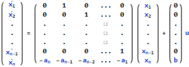
 =Ax+Bu ……….(13)
Note: Matrix A is known as Bush form or companion form. Matrix B has all elements zero except the last element.

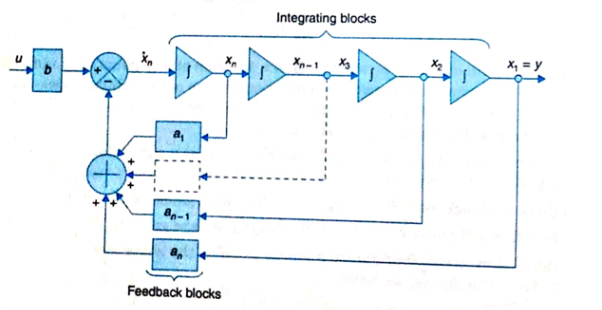
The output equation is given as y=x1
y=Cx ……….(14)
Where C = [1 0 0………..0]

Fig2: State model
The above figure shows the state model of a system with two inputs u1(t) and u2(t), and having outputs y1(t) and y2(t). As discussed in above section 5.1, we know that the output equation is given as
Y(t)=Cx(t)+Du(t) (9)
 (10)
(10)
Taking L.T of equation (9)
Y(s)=CX(s)+DU(s) (11)
Taking L.T of equation (10)
SX(s)=AX(s)+BU(s) (12)
X(s)=[SI-A]-1BU(s) (13)
Y(s)=CX(s)+DU(s)
Y(s)=C{[SI-A]-1BU(s)} + DU(s)
 (14)
(14)

The denominator of equation (14) is the characteristic equation
[SI-A]=0
The state variables selected here are the physical quantities of the system, which can be measured. The selection of these variables can be directly related to the physical system because the solution of the state equation is related to the time variation of the system variables.
The number of energy storing elements in any system is equal to the number of state variables. Below shown are few electrical circuits, just to brush up on the concept of energy storing elements and state variable relation.
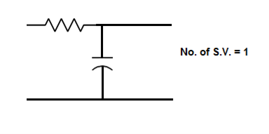

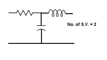
Fig 3 Electrical circuit with energy storing elements
Now calculating the state equation and output equation for state variable analysis.
State Equation and Output equation:
Number of output=Number of output equation

Fig 4 State Model
Considering multiple input and multiple output system, with two inputs u1(t)and u2(t), and two outputs y1(t) and y2(t) respectively.
y1(t)=c11x1(t)+c12x2(t)+d11u1(t)+d12u2(t)
y2(t)=c21x1(t)+c22x2(t)+d21u1(t)+d22u2(t)

The output equation is given as
Y(t)=CX(t)+DU(t)


# Now finding State Equation
Number of energy-storing elements= Number of state variables

=a11x1(t)+a12x2(t)+b11u1(t)+b12u2(t)

=a21x1(t)+a22x2(t)+b21u1(t)+b22u2(t)

The state equation is then given as
 =Ax(t)+Bu(t)
Key takeaway
The number of energy storing element= Number of state variables
We should always take voltage across the inductor L, and current through capacitor C.
Question: Obtain the state space representation for the given electrical system
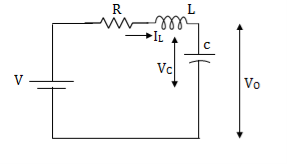
Solution: The state model is given as

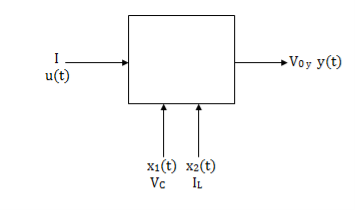
The state model shows that there are two energy storing elements L, C. As we already know that Number of state variables is equal to the number of energy storing elements. Hence we have two state variables[x1(t) and x2(t)]. We have one output V0(taken across the capacitor) and input u(t).
The output equation is then given as
Y(t)=CX(t)+DU(t)
V0=Vc= x1(t) ….(a)
Hence output equation becomes
V0= x1(t)
y(t)=[1 0]  +[0]u(t)
So, C=[1 0] D=[0]
Now writing the state equation
 =Ax(t)+Bu(t)
For that applying KVL in the above circuit
V=ILR+L +Vc
+Vc
State Equation is  =Ax(t)+Bu(t)
 =
=
x1(t)=Vc
 =
=
IL=C
 =
=
 =
= =
=
 =(1/C) x2(t) ……….(b)
 =
= =
=
VL=L
 =
= =VL/L
=VL/L
From KVL
L =VL=V-ILR-VC
 =
= =
=
 =
= …………….(c)
From equation (b) and (c)
 = [0 1/c]
  + [0 0]u(t)
 =[-1/L -R/L]
  + [1/L 0]
Now writing the state equation
 =Ax(t)+Bu(t)

Hence


Question: Obtain the state space representation for the given electrical system
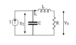
Solution: The state model shows that there are two energy storing elements L, C. As we already know that Number of state variables is equal to the number of energy storing elements. Hence we have two state variables[x1(t) and x2(t)]. We have one output V0(taken across the capacitor) and input u(t).
Here output is V0. But from above electrical circuit V0=ILR
V0=x2(t)R
y(t)= V0= [0 R]  + [0] u(t)
The output equation is given as
Y(t)=CX(t)+DU(t)
C=[0 R] D=[0]
Now finding state equation,we apply KCL in the given electrical circuit
I=IC+IL
 =
=
But I-IL=IC
 =
=
 =
=
 =
=
 =
= x2(t)+
 ……..(a)
 =[0 1/C]
 + [1/C 0]
 …….(b)
 =
= =
=
Applying KVL in the given electrical circuit we get
VC=VL+ILR
VC-ILR=VL=L

 =
=
 = [1/L -R/L]
  + [0] u(t) …………. (c)
From equation (b) and (c) we have
Now writing the state equation
 =Ax(t)+Bu(t)
 =
= +
+ 
Hence A= B=
B= 
Note: We should always take voltage across the inductor L, and current through capacitor C.
References:
1. Control Systems Engineering, I.J. Nagrath, M. Gopal
2. Modern Control system (II Edition) – Katsuhiko Ogata
3. Control systems by Smarajit Ghosh (second Edition, Pearson Education)
Unit - 6
State variable methods of analysis
The state of a system is a minimal set of variables known as state variables. The knowledge of these variables at any instance of time together with the knowledge of the inputs for the same instance of time determines the complete behaviour of the system. The fewer drawbacks in the transfer function method for representing any system led to the use of state variables in the analysis of the system. Few advantages are listed below:
- The state-space can be used for linear or nonlinear, time-variant, or time-invariant systems.
- It is easier to apply where Laplace transform cannot be applied.
- The nth order differential equation can be expressed as the 'n' equation of the first order.
- It is a time-domain method.
- As this is a time-domain method, therefore this method is suitable for digital computer computation.
- Based on the given performance index, this system can be designed for optimal conditions.
Representation of state-space: The system shown below has ‘m’ inputs, ‘p, outputs, and ‘n’ number of state variables. The state equation gives us the relation between the state variables and the inputs.

Fig 1 State variable
So, the above system shown can be described through equations as
 =f1 (x1, x2,…….xn , u1, u2……… ,um)
 = f2 (x1, x2,…….xn , u1, u2……… ,um)
 =f1 (x1, x2,…….xn , u1, u2……… ,um) (1)
The above set of equations can be represented as
 =f(x(t),u(t)) (2)
As we are concerned for time invariant system, for which the term  in (1) is a linear combination of state variables and input. So,
 (t)=2tx1+x2+u1+u2 (3)
 =a11x1(t)+a12x2(t)+…a1nxn(t)+b11u1(t)+b12u2(t)+…….+b1mum(t)
 =a21x1(t)+a22x2(t)+…a2nxn(t)+b21u1(t)+b22u2(t)+…….+b2mum(t)
 =an1x1(t)+an2x2(t)+…annxn(t)+bn1u1(t)+bn2u2(t)+…….+bnmum(t)
The above equation can be represented in matrix form as given below
 (4)
(4)
The above coefficients aij and bji in equation (4) can be written in a vector-matrix form as
 =Ax(t)+Bu(t) (5)
Key takeaway
The state of a system is a minimal set of variables known as state variables.
The vector-matrix form is given as  =Ax(t)+Bu(t)
As their name implies, state variable models are based on the concept of a system’s state. The state of a system is the minimum amount of information necessary to completely characterize the system at some instant in time. It turns out that the system’s state provides the information necessary to uniquely determine the energy in all the system’s energy storage elements and vice-versa. If the energy in any of the energy storage elements changes, the system’s state changes. The state variables are the smallest set of variables which completely describe the state (or the energy storage) of the system. The choice of state variables is not unique, but one possible choice of state variable is those variables which describe the energy stored in all of the independent energy storage elements in the system. For example, in electrical circuits, inductors store energy as current and capacitors store energy as voltage. If we choose as state variables the currents in inductors and the voltages across the capacitors, we will have created a legitimate set of state variables for the circuit. Since the state variables are independent, they can be visualized as a set of orthogonal axes defining a space. The space defined by the state variables is called state space of the system. If the system is described by N state variables, the state space will be N-dimensional. The state of the system at any given time can be visualized as a point in the state space. In general, as we apply an input to a system, the system’s state will change over time. Since the state of the system is a point in state space, the change in the system’s state can be visualized as tracing a path over time in the state space. This path is called the state trajectory.
6.4 Representation of vector matrix differential Equation
Solution of homogeneous state equation
The first order differential equation is given as
 =ax x(0)=x0
x(t)= x0=
x0=
Consider state equation
 =Ax(t); x(0)=x0
The solution will be of the form
x(t)=a0+a1t+a2t2+a3t3+….+aiti
Substituting value in above equation
a1+2a2t2+3a3t3+……….=A[a0+a1t+a2t2+a3t3+….+aiti]
a1=Aa0
a2= Aa1=
Aa1= A2a0
A2a0
ai= Aia0
Aia0
Solution for x(t) will be
x(t)=[I+At+ A2t2+………+
 Aiti]x0
The matrix exponential form can be written as

The solution x(t) will be x(t)= x0
x0
 =Ax(t)+Bu(t) and x(0)=x0
 - Ax(t)=Bu(t)
Multiplying both sides by 
 [
[ - Ax(t)]=
 =
= Bu(t)
Bu(t)
Integrating both sides w.r.t t we get
 =
=  d
d
 =
= d
d
Multiplying both sides by 
x(t)= x(0)+
x(0)+ d
d
 x(0) is called as Homogeneous solution
 d
d is the Forced solution
At t=t0
x(t)= x(t0)+
 d
d
The above equation is the required solution.
Solution of non-homogeneous state equation
Let the scalar state equation be
 =ax+bu
 -ax=bu
Multiplying both sides by e-at
x(t) = eat x(0) + d
d
Then for non-homogeneous state equation
 =Ax+Bu
The solution x(t) can be given as
x(t) = eAt x(0) + d
d
The above equation is the required solution.
Key takeaway
Solution of homogeneous state equation
x(t)= x(t0)+
 d
d
Solution of non-homogeneous state equation
x(t) = eAt x(0) + d
d
nth order differential equation and transfer function
The phase variables are defined as the state variables obtained from any one of the system variables and its derivatives. The nth order linear differential equation for given input y(t) and output u(t) is given as
y(n)+a1y(n-1)+………..+an-1 +any=bou(m)+……+bm-1
 + bm u. ….. (9)
The initial conditions are expressed as y(0), ,…..,y(n-1)(0).
The transfer function assuming all initial conditions zero is
T(s)= =[b0sm+b1sm-1+….+bm-1s+bm/[sn+a1sn-1+……..+an-1s+an] ……(10)
Considering simple case when there are no zeros in the system, the transfer function becomes
T(s)= =[b]/ [sn+a1sn-1+……..+an-1s+an] …….(11)
For above transfer function the differential equation is given as
y(n)+a1y(n-1)+………..+an-1 +any=b u …….(12)
Let x1=y
x2=
…….
xn=y(n-1)
From (12) the differential equation is given as


……….

 =-anx1-an-1x2-…….-a1xn+bu
 =Ax+Bu ……….(13)
Note: Matrix A is known as Bush form or companion form. Matrix B has all elements zero except the last element.
The output equation is given as y=x1
y=Cx ……….(14)
Where C = [1 0 0………..0]

Fig2: State model
The above figure shows the state model of a system with two inputs u1(t) and u2(t), and having outputs y1(t) and y2(t). As discussed in above section 5.1, we know that the output equation is given as
Y(t)=Cx(t)+Du(t) (9)
 (10)
(10)
Taking L.T of equation (9)
Y(s)=CX(s)+DU(s) (11)
Taking L.T of equation (10)
SX(s)=AX(s)+BU(s) (12)
X(s)=[SI-A]-1BU(s) (13)
Y(s)=CX(s)+DU(s)
Y(s)=C{[SI-A]-1BU(s)} + DU(s)
 (14)
(14)

The denominator of equation (14) is the characteristic equation
[SI-A]=0
The state variables selected here are the physical quantities of the system, which can be measured. The selection of these variables can be directly related to the physical system because the solution of the state equation is related to the time variation of the system variables.
The number of energy storing elements in any system is equal to the number of state variables. Below shown are few electrical circuits, just to brush up on the concept of energy storing elements and state variable relation.


Fig 3 Electrical circuit with energy storing elements
Now calculating the state equation and output equation for state variable analysis.
State Equation and Output equation:
Number of output=Number of output equation
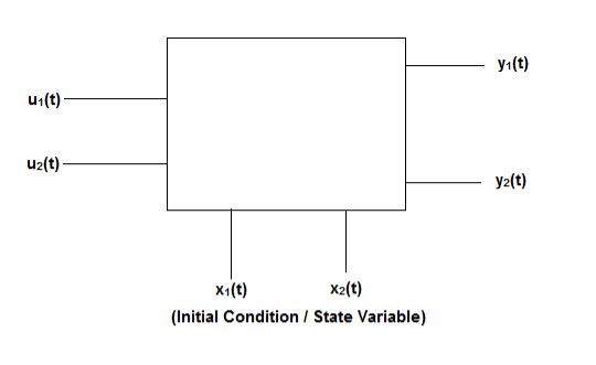
Fig 4 State Model
Considering multiple input and multiple output system, with two inputs u1(t)and u2(t), and two outputs y1(t) and y2(t) respectively.
y1(t)=c11x1(t)+c12x2(t)+d11u1(t)+d12u2(t)
y2(t)=c21x1(t)+c22x2(t)+d21u1(t)+d22u2(t)

The output equation is given as
Y(t)=CX(t)+DU(t)


# Now finding State Equation
Number of energy-storing elements= Number of state variables

=a11x1(t)+a12x2(t)+b11u1(t)+b12u2(t)

=a21x1(t)+a22x2(t)+b21u1(t)+b22u2(t)

The state equation is then given as
 =Ax(t)+Bu(t)
Key takeaway
The number of energy storing element= Number of state variables
We should always take voltage across the inductor L, and current through capacitor C.
Question: Obtain the state space representation for the given electrical system

Solution: The state model is given as

The state model shows that there are two energy storing elements L, C. As we already know that Number of state variables is equal to the number of energy storing elements. Hence we have two state variables[x1(t) and x2(t)]. We have one output V0(taken across the capacitor) and input u(t).
The output equation is then given as
Y(t)=CX(t)+DU(t)
V0=Vc= x1(t) ….(a)
Hence output equation becomes
V0= x1(t)
y(t)=[1 0]  +[0]u(t)
So, C=[1 0] D=[0]
Now writing the state equation
 =Ax(t)+Bu(t)
For that applying KVL in the above circuit
V=ILR+L +Vc
+Vc
State Equation is  =Ax(t)+Bu(t)
 =
=
x1(t)=Vc
 =
=
IL=C
 =
=
 =
= =
=
 =(1/C) x2(t) ……….(b)
 =
= =
=
VL=L
 =
= =VL/L
=VL/L
From KVL
L =VL=V-ILR-VC
 =
= =
=
 =
= …………….(c)
From equation (b) and (c)
 = [0 1/c]
  + [0 0]u(t)
 =[-1/L -R/L]
  + [1/L 0]
Now writing the state equation
 =Ax(t)+Bu(t)

Hence


Question: Obtain the state space representation for the given electrical system

Solution: The state model shows that there are two energy storing elements L, C. As we already know that Number of state variables is equal to the number of energy storing elements. Hence we have two state variables[x1(t) and x2(t)]. We have one output V0(taken across the capacitor) and input u(t).

Here output is V0. But from above electrical circuit V0=ILR
V0=x2(t)R
y(t)= V0= [0 R]  + [0] u(t)
The output equation is given as
Y(t)=CX(t)+DU(t)
C=[0 R] D=[0]
Now finding state equation,we apply KCL in the given electrical circuit
I=IC+IL
 =
=
But I-IL=IC
 =
=
 =
=
 =
=
 =
= x2(t)+
 ……..(a)
 =[0 1/C]
 + [1/C 0]
 …….(b)
 =
= =
=
Applying KVL in the given electrical circuit we get
VC=VL+ILR
VC-ILR=VL=L

 =
=
 = [1/L -R/L]
  + [0] u(t) …………. (c)
From equation (b) and (c) we have
Now writing the state equation
 =Ax(t)+Bu(t)
 =
= +
+ 
Hence A= B=
B= 
Note: We should always take voltage across the inductor L, and current through capacitor C.
References:
1. Control Systems Engineering, I.J. Nagrath, M. Gopal
2. Modern Control system (II Edition) – Katsuhiko Ogata
3. Control systems by Smarajit Ghosh (second Edition, Pearson Education)
Unit - 6
State variable methods of analysis
The state of a system is a minimal set of variables known as state variables. The knowledge of these variables at any instance of time together with the knowledge of the inputs for the same instance of time determines the complete behaviour of the system. The fewer drawbacks in the transfer function method for representing any system led to the use of state variables in the analysis of the system. Few advantages are listed below:
- The state-space can be used for linear or nonlinear, time-variant, or time-invariant systems.
- It is easier to apply where Laplace transform cannot be applied.
- The nth order differential equation can be expressed as the 'n' equation of the first order.
- It is a time-domain method.
- As this is a time-domain method, therefore this method is suitable for digital computer computation.
- Based on the given performance index, this system can be designed for optimal conditions.
Representation of state-space: The system shown below has ‘m’ inputs, ‘p, outputs, and ‘n’ number of state variables. The state equation gives us the relation between the state variables and the inputs.

Fig 1 State variable
So, the above system shown can be described through equations as
 =f1 (x1, x2,…….xn , u1, u2……… ,um)
 = f2 (x1, x2,…….xn , u1, u2……… ,um)
 =f1 (x1, x2,…….xn , u1, u2……… ,um) (1)
The above set of equations can be represented as
 =f(x(t),u(t)) (2)
As we are concerned for time invariant system, for which the term  in (1) is a linear combination of state variables and input. So,
 (t)=2tx1+x2+u1+u2 (3)
 =a11x1(t)+a12x2(t)+…a1nxn(t)+b11u1(t)+b12u2(t)+…….+b1mum(t)
 =a21x1(t)+a22x2(t)+…a2nxn(t)+b21u1(t)+b22u2(t)+…….+b2mum(t)
 =an1x1(t)+an2x2(t)+…annxn(t)+bn1u1(t)+bn2u2(t)+…….+bnmum(t)
The above equation can be represented in matrix form as given below
 (4)
(4)
The above coefficients aij and bji in equation (4) can be written in a vector-matrix form as
 =Ax(t)+Bu(t) (5)
Key takeaway
The state of a system is a minimal set of variables known as state variables.
The vector-matrix form is given as  =Ax(t)+Bu(t)
As their name implies, state variable models are based on the concept of a system’s state. The state of a system is the minimum amount of information necessary to completely characterize the system at some instant in time. It turns out that the system’s state provides the information necessary to uniquely determine the energy in all the system’s energy storage elements and vice-versa. If the energy in any of the energy storage elements changes, the system’s state changes. The state variables are the smallest set of variables which completely describe the state (or the energy storage) of the system. The choice of state variables is not unique, but one possible choice of state variable is those variables which describe the energy stored in all of the independent energy storage elements in the system. For example, in electrical circuits, inductors store energy as current and capacitors store energy as voltage. If we choose as state variables the currents in inductors and the voltages across the capacitors, we will have created a legitimate set of state variables for the circuit. Since the state variables are independent, they can be visualized as a set of orthogonal axes defining a space. The space defined by the state variables is called state space of the system. If the system is described by N state variables, the state space will be N-dimensional. The state of the system at any given time can be visualized as a point in the state space. In general, as we apply an input to a system, the system’s state will change over time. Since the state of the system is a point in state space, the change in the system’s state can be visualized as tracing a path over time in the state space. This path is called the state trajectory.
6.4 Representation of vector matrix differential Equation
Solution of homogeneous state equation
The first order differential equation is given as
 =ax x(0)=x0
x(t)= x0=
x0=
Consider state equation
 =Ax(t); x(0)=x0
The solution will be of the form
x(t)=a0+a1t+a2t2+a3t3+….+aiti
Substituting value in above equation
a1+2a2t2+3a3t3+……….=A[a0+a1t+a2t2+a3t3+….+aiti]
a1=Aa0
a2= Aa1=
Aa1= A2a0
A2a0
ai= Aia0
Aia0
Solution for x(t) will be
x(t)=[I+At+ A2t2+………+
 Aiti]x0
The matrix exponential form can be written as

The solution x(t) will be x(t)= x0
x0
 =Ax(t)+Bu(t) and x(0)=x0
 - Ax(t)=Bu(t)
Multiplying both sides by 
 [
[ - Ax(t)]=
 =
= Bu(t)
Bu(t)
Integrating both sides w.r.t t we get
 =
=  d
d
 =
= d
d
Multiplying both sides by 
x(t)= x(0)+
x(0)+ d
d
 x(0) is called as Homogeneous solution
 d
d is the Forced solution
At t=t0
x(t)= x(t0)+
 d
d
The above equation is the required solution.
Solution of non-homogeneous state equation
Let the scalar state equation be
 =ax+bu
 -ax=bu
Multiplying both sides by e-at
x(t) = eat x(0) + d
d
Then for non-homogeneous state equation
 =Ax+Bu
The solution x(t) can be given as
x(t) = eAt x(0) + d
d
The above equation is the required solution.
Key takeaway
Solution of homogeneous state equation
x(t)= x(t0)+
 d
d
Solution of non-homogeneous state equation
x(t) = eAt x(0) + d
d
nth order differential equation and transfer function
The phase variables are defined as the state variables obtained from any one of the system variables and its derivatives. The nth order linear differential equation for given input y(t) and output u(t) is given as
y(n)+a1y(n-1)+………..+an-1 +any=bou(m)+……+bm-1
 + bm u. ….. (9)
The initial conditions are expressed as y(0), ,…..,y(n-1)(0).
The transfer function assuming all initial conditions zero is
T(s)= =[b0sm+b1sm-1+….+bm-1s+bm/[sn+a1sn-1+……..+an-1s+an] ……(10)
Considering simple case when there are no zeros in the system, the transfer function becomes
T(s)= =[b]/ [sn+a1sn-1+……..+an-1s+an] …….(11)
For above transfer function the differential equation is given as
y(n)+a1y(n-1)+………..+an-1 +any=b u …….(12)
Let x1=y
x2=
…….
xn=y(n-1)
From (12) the differential equation is given as


……….

 =-anx1-an-1x2-…….-a1xn+bu

 =Ax+Bu ……….(13)
Note: Matrix A is known as Bush form or companion form. Matrix B has all elements zero except the last element.

The output equation is given as y=x1
y=Cx ……….(14)
Where C = [1 0 0………..0]
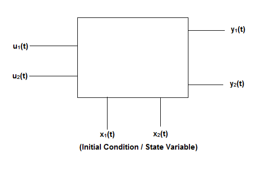
Fig2: State model
The above figure shows the state model of a system with two inputs u1(t) and u2(t), and having outputs y1(t) and y2(t). As discussed in above section 5.1, we know that the output equation is given as
Y(t)=Cx(t)+Du(t) (9)
 (10)
(10)
Taking L.T of equation (9)
Y(s)=CX(s)+DU(s) (11)
Taking L.T of equation (10)
SX(s)=AX(s)+BU(s) (12)
X(s)=[SI-A]-1BU(s) (13)
Y(s)=CX(s)+DU(s)
Y(s)=C{[SI-A]-1BU(s)} + DU(s)
 (14)
(14)

The denominator of equation (14) is the characteristic equation
[SI-A]=0
The state variables selected here are the physical quantities of the system, which can be measured. The selection of these variables can be directly related to the physical system because the solution of the state equation is related to the time variation of the system variables.
The number of energy storing elements in any system is equal to the number of state variables. Below shown are few electrical circuits, just to brush up on the concept of energy storing elements and state variable relation.

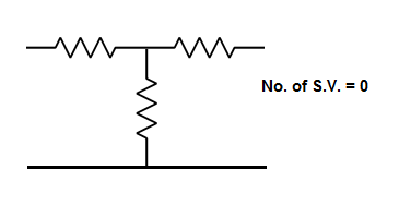

Fig 3 Electrical circuit with energy storing elements
Now calculating the state equation and output equation for state variable analysis.
State Equation and Output equation:
Number of output=Number of output equation

Fig 4 State Model
Considering multiple input and multiple output system, with two inputs u1(t)and u2(t), and two outputs y1(t) and y2(t) respectively.
y1(t)=c11x1(t)+c12x2(t)+d11u1(t)+d12u2(t)
y2(t)=c21x1(t)+c22x2(t)+d21u1(t)+d22u2(t)

The output equation is given as
Y(t)=CX(t)+DU(t)


# Now finding State Equation
Number of energy-storing elements= Number of state variables

=a11x1(t)+a12x2(t)+b11u1(t)+b12u2(t)

=a21x1(t)+a22x2(t)+b21u1(t)+b22u2(t)

The state equation is then given as
 =Ax(t)+Bu(t)
Key takeaway
The number of energy storing element= Number of state variables
We should always take voltage across the inductor L, and current through capacitor C.
Question: Obtain the state space representation for the given electrical system

Solution: The state model is given as

The state model shows that there are two energy storing elements L, C. As we already know that Number of state variables is equal to the number of energy storing elements. Hence we have two state variables[x1(t) and x2(t)]. We have one output V0(taken across the capacitor) and input u(t).
The output equation is then given as
Y(t)=CX(t)+DU(t)
V0=Vc= x1(t) ….(a)
Hence output equation becomes
V0= x1(t)
y(t)=[1 0]  +[0]u(t)
So, C=[1 0] D=[0]
Now writing the state equation
 =Ax(t)+Bu(t)
For that applying KVL in the above circuit
V=ILR+L +Vc
+Vc
State Equation is  =Ax(t)+Bu(t)
 =
=
x1(t)=Vc
 =
=
IL=C
 =
=
 =
= =
=
 =(1/C) x2(t) ……….(b)
 =
= =
=
VL=L
 =
= =VL/L
=VL/L
From KVL
L =VL=V-ILR-VC
 =
= =
=
 =
= …………….(c)
From equation (b) and (c)
 = [0 1/c]
  + [0 0]u(t)
 =[-1/L -R/L]
  + [1/L 0]
Now writing the state equation
 =Ax(t)+Bu(t)

Hence


Question: Obtain the state space representation for the given electrical system

Solution: The state model shows that there are two energy storing elements L, C. As we already know that Number of state variables is equal to the number of energy storing elements. Hence we have two state variables[x1(t) and x2(t)]. We have one output V0(taken across the capacitor) and input u(t).

Here output is V0. But from above electrical circuit V0=ILR
V0=x2(t)R
y(t)= V0= [0 R]  + [0] u(t)
The output equation is given as
Y(t)=CX(t)+DU(t)
C=[0 R] D=[0]
Now finding state equation,we apply KCL in the given electrical circuit
I=IC+IL
 =
=
But I-IL=IC
 =
=
 =
=
 =
=
 =
= x2(t)+
 ……..(a)
 =[0 1/C]
 + [1/C 0]
 …….(b)
 =
= =
=
Applying KVL in the given electrical circuit we get
VC=VL+ILR
VC-ILR=VL=L

 =
=
 = [1/L -R/L]
  + [0] u(t) …………. (c)
From equation (b) and (c) we have
Now writing the state equation
 =Ax(t)+Bu(t)
 =
= +
+ 
Hence A= B=
B= 
Note: We should always take voltage across the inductor L, and current through capacitor C.
References:
1. Control Systems Engineering, I.J. Nagrath, M. Gopal
2. Modern Control system (II Edition) – Katsuhiko Ogata
3. Control systems by Smarajit Ghosh (second Edition, Pearson Education)