Unit - 3
Linked List- Linked List as ADT
Dynamic memory allocation is the process of allocating memory at runtime. Memory management functions are library routines that are used to allocate and free memory during the execution of a programme. The stdlib.h header file defines these functions.
● malloc() - returns a void pointer referring to the first byte of the allocated space after allocating the required size of bytes.
● calloc() - Returns a void pointer to the memory after allocating space for an array of items and initializing them to zero.
● free - Memory that had previously been assigned is released.
● realloc - change the size of a previously assigned space
Malloc()
The malloc() function in C is used to allocate memory. It is a function that is used to dynamically allocate a block of memory. It sets aside a given amount of memory space and returns a null reference to the memory address. Typically, the pointer returned is of type void. It means that any pointer can be assigned to the C malloc() function.
The malloc() function has the following syntax:
Ptr = (cast_type *) malloc (byte_size);
Here,
● ptr is a pointer of cast_type.
● The C malloc() function returns a pointer to the allocated memory of byte_size.
Free()
At compile time, the memory for variables is automatically deallocated. You must explicitly deallocate memory in dynamic memory allocation. You might get an out of memory error if you don't do it.
In C, the free() function is used to free/deallocate memory. You can make additional memory available for later usage by releasing memory in your software.
Example
#include <stdio.h>
Int main() {
Int* ptr = malloc(10 * sizeof(*ptr));
If (ptr != NULL){
*(ptr + 2) = 50;
printf("Value of the 2nd integer is %d",*(ptr + 2));
}
Free(ptr);
}
Output
Value of the 2nd integer is 50
Calloc()
Contiguous allocation is represented by the C calloc() function. This function is used to allocate memory in numerous blocks. It's a dynamic memory allocation function that handles memory allocation for complex data structures like arrays and structures.
The malloc() function allocates a single block of memory, whereas the calloc() function in C allocates many blocks of memory. The calloc() function allocates blocks of the same size to each user.
The calloc() function has the following syntax:
Ptr = (cast_type *) calloc (n, size);
● The above statement is used to allocate n identical memory chunks.
● After the memory area has been allocated, all bytes are set to zero.
● Returns the pointer that is now at the first byte of the allocated memory region.
Example
#include <stdio.h>
int main() {
int i, * ptr, sum = 0;
ptr = calloc(10, sizeof(int));
if (ptr == NULL) {
printf("Error! memory not allocated.");
exit(0);
}
printf("Building and calculating the sequence sum of the first 10 terms \ n ");
for (i = 0; i < 10; ++i) { * (ptr + i) = i;
sum += * (ptr + i);
}
printf("Sum = %d", sum);
free(ptr);
return 0;
}
Result:
Building and calculating the sequence sum of the first 10 terms
Sum = 45
Difference between malloc() and calloc()
Calloc() | Malloc() |
Calloc() sets the value of the allocated memory to zero. | Malloc() allocates memory and fills it with trash values. |
The total number of arguments is two. | There is just one argument. |
Syntax : (cast_type *)calloc(blocks , size_of_block); | Syntax : (cast_type *)malloc(Size_in_bytes); |
In programming, it is the most widely used linked list. When we talk about a linked list, we're talking about a singly linked list. The singly linked list is a data structure that is divided into two parts: the data portion and the address part, which contains the address of the next or successor node. A pointer is another name for the address component of a node.
Assume we have three nodes with addresses of 100, 200, and 300, respectively. The following diagram depicts the representation of three nodes as a linked list:

Fig 1: Singly linked list
In the diagram above, we can see three separate nodes with addresses of 100, 200, and 300, respectively. The first node has the address of the next node, which is 200, the second has the address of the last node, which is 300, and the third has the NULL value in its address portion because it does not point to any node. A head pointer is a pointer that stores the address of the first node.
Because there is just one link in the linked list depicted in the figure, it is referred to as a singly linked list. Just forward traversal is permitted in this list; we can't go backwards because there is only one link in the list.
Representation of the node in a singly linked list
Struct node
{
int data;
struct node *next;
}
In the above diagram, we've constructed a user-made structure called a node, which has two members: one is data of integer type, and the other is the node type's pointer (next).
Doubly linked list
The doubly linked list, as its name implies, has two pointers. The doubly linked list can be described as a three-part linear data structure: the data component, the address part, and the other two address parts. A doubly linked list, in other terms, is a list with three parts in each node: one data portion, a pointer to the previous node, and a pointer to the next node.
Let's pretend we have three nodes with addresses of 100, 200, and 300, respectively. The representation of these nodes in a doubly-linked list is shown below:

Fig 2: Doubly linked list
The node in a doubly-linked list contains two address portions, as shown in the diagram above; one part keeps the address of the next node, while the other half stores the address of the previous node. The address component of the first node in the doubly linked list is NULL, indicating that the prior node's address is NULL.
Representation of the node in a doubly linked list
Struct node
{
int data;
struct node *next;
Struct node *prev;
}
In the above representation, we've constructed a user-defined structure called a node, which has three members: one is data of integer type, and the other two are pointers of the node type, i.e. next and prev. The address of the next node is stored in the next pointer variable, whereas the address of the previous node is stored in the prev pointer variable. The type of both the pointers, i.e., next and prev is struct node as both the pointers are storing the address of the node of the struct node type.
Circular linked list
A singly linked list is a type of circular linked list. The sole difference between a singly linked list and a circular linked list is that the last node in a singly linked list does not point to any other node, therefore its link portion is NULL. The circular linked list, on the other hand, is a list in which the last node connects to the first node, and the address of the first node is stored in the link section of the last node.
There are no nodes at the beginning or finish of the circular linked list. We can travel in either way, backwards or forwards. The following is a diagrammatic illustration of the circular linked list:
Struct node
{
int data;
struct node *next;
}
A circular linked list is a collection of elements in which each node is linked to the next and the last node is linked to the first. The circular linked list will be represented similarly to the singly linked list, as demonstrated below:
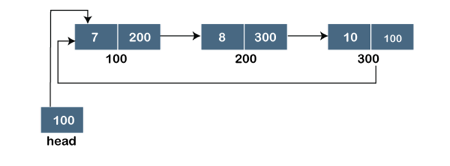
Fig 3: Circular linked list
Key takeaway
- The singly linked list is a data structure that is divided into two parts: the data portion and the address part, which contains the address of the next or successor node.
- A pointer is another name for the address component of a node.
- The doubly linked list can be described as a three-part linear data structure: the data component, the address part, and the other two address parts.
- The circular linked list, on the other hand, is a list in which the last node connects to the first node, and the address of the first node is stored in the link section of the last node.
Let's look at how each linked list node is represented. Each node is made up of the following components:
● A data point.
● Another node's address.
We use a struct to package both the data item and the next node reference, as follows:
Struct node
{
int data;
struct node *next;
};
The key to grasping a linked list node's structure is to understand its structure.
A data item and a pointer to another struct node are both present in each struct node. To see how this works, let's make a basic Linked List with three items.
/* Initialize nodes */
Struct node *head;
Struct node *one = NULL;
Struct node *two = NULL;
Struct node *three = NULL;
/* Allocate memory */
One = malloc(sizeof(struct node));
Two = malloc(sizeof(struct node));
Three = malloc(sizeof(struct node));
/* Assign data values */
One->data = 1;
Two->data = 2;
Three->data=3;
/* Connect nodes */
One->next = two;
Two->next = three;
Three->next = NULL;
/* Save address of first node in head */
Head = one;
All you need is a review on pointers and structs if you didn't comprehend any of the lines above.
We've developed a simple linked list with three nodes in only a few steps.

The capacity to break and rejoin a linked list is what gives it its power. For example, if you wanted to place element 4 between 1 and 2, you would do so as follows:
● Make a new struct node and give it some memory.
● Add 4 to the data value.
● Set the next pointer to the struct node with the data value of 2 as the data value.
● Change the "1"'s next pointer to the node we just made.
Insertion
When placing a node into a linked list, there are three possible scenarios:
● Insertion at the beginning
● Insertion at the end. (Append)
● Insertion after a given node
Insertion at the beginning
There's no need to look for the end of the list. If the list is empty, the new node becomes the list's head. Otherwise, we must connect the new node to the existing list's head and make the new node the list's head.
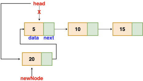
Fig 4: Insertion at beginning
// function is returning the head of the singly linked-list
Node insertAtBegin(Node head, int val)
{
newNode = new Node(val) // creating new node of linked list
if(head == NULL) // check if linked list is empty
return newNode
else // inserting the node at the beginning
{
newNode.next = head
return newNode
}
}
Insertion at the end
We'll go through the list till we reach the last node. The new node is then appended to the end of the list. It's worth noting that there are some exceptions, such as when the list is empty.
We will return the updated head of the linked list if the list is empty, because the inserted node is both the first and end node of the linked list in this case.
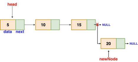
Fig 5: Insertion at end
// the function is returning the head of the singly linked list
Node insertAtEnd(Node head, int val)
{
if( head == NULL ) // handing the special case
{
newNode = new Node(val)
head = newNode
return head
}
Node temp = head
// traversing the list to get the last node
while( temp.next != NULL )
{
temp = temp.next
}
newNode = new Node(val)
temp.next = newNode
return head
}
Insertion after a given node
The reference to a node is passed to us, and the new node is put after it.
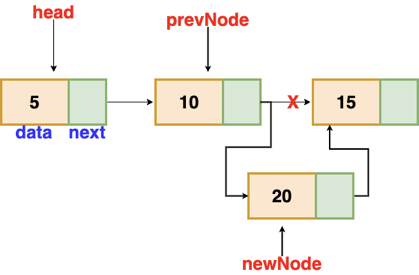
Fig 6: Insertion after given node
Void insertAfter(Node prevNode, int val)
{
newNode = new Node(val)
newNode.next = prevNode.next
prevNode.next = newNode
}
Deletion
These are the procedures to delete a node from a linked list.
● Find the previous node of the node to be deleted.
● Change the next pointer of the previous node
● Free the memory of the deleted node.
There is a specific circumstance in which the first node is removed upon deletion. We must update the connected list's head in this case.

Fig 7: Deleting a node in linked list
// this function will return the head of the linked list
Node deleteLL(Node head, Node del)
{
if(head == del) // if the node to be deleted is the head node
{
return head.next // special case for the first Node
}
Node temp = head
while( temp.next != NULL )
{
if(temp.next == del) // finding the node to be deleted
{
temp.next = temp.next.next
delete del // free the memory of that Node
return head
}
temp = temp.next
}
return head // if no node matches in the Linked List
}
Traversal
The goal is to work your way through the list from start to finish. We might want to print the list or search for a certain node in it, for example.
The traversal algorithm for a list
● Start with the head of the list. Access the content of the head node if it is not null.
● Then go to the next node(if exists) and access the node information
● Continue until no more nodes (that is, you have reached the null node)
Void traverseLL(Node head) {
while(head != NULL)
{
print(head.data)
head = head.next
}
}
Key takeaway
- There's no need to look for the end of the list. If the list is empty, the new node becomes the list's head.
- The goal is to work your way through the list from start to finish. We might want to print the list or search for a certain node in it.
Polynomials can be represented in a number of different ways. These are the following:
● By the use of arrays
● By the use of Linked List
Representation of polynomial using Arrays
There may be times when you need to evaluate a large number of polynomial expressions and execute fundamental arithmetic operations on them, such as addition and subtraction. You'll need a mechanism to express the polynomials for this. The simplest method is to express a polynomial of degree 'n' and store the coefficient of the polynomial's n+1 terms in an array. As a result, each array element will have two values:
● Coefficient and
● Exponent
Polynomial of representation using linked lists
An ordered list of non-zero terms can be thought of as a polynomial. Each non-zero word is a two-tuple, containing two pieces of data:
● The exponent part
● The coefficient part
Multiplication
To multiply two polynomials, multiply the terms of one polynomial by the terms of the other polynomial. Assume the two polynomials have n and m terms respectively. A polynomial with n times m terms will be created as a result of this method.
For example, we can construct a linked list by multiplying 2 – 4x + 5x2 and 1 + 2x – 3x3:
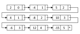
All of the terms we'll need to get the final outcome are in this linked list. The powers, on the other hand, do not sort it. It also has duplicate nodes with similar terms. We can merge sort the linked list depending on each node's power to get the final linked list:
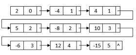
After sorting, the nodes with similar terms are clustered together. Then, for the final multiplication result, we can combine each set of like terms:

Addition
We can combine two polynomials by adding the coefficients of related expressions and creating a new linked list for the resultant polynomial. Polynomials 2 – 4x + 5x2 and 1 + 2x – 3x3, for example, can be represented with two favourite lists.

When we add them up, we may group the phrases that are similar and get the result 3 – 2x2 + 5x2 – 3x3.

We may use a two-pointer approach to merge the two sorted linked lists because they are both ordered by power:

We first generate two pointers, p1 and p2, to the head pointers of the two input polynomials in this algorithm. Then, using the powers of these two pointers, we build new polynomial nodes. There are three possibilities:
● p1‘s power is greater than p2‘s power: In this case, we append a new node with p1‘s power and coefficient. Also, we move p1 to the next node.
● p2‘s power is greater than p1‘s power: In this case, we append a new node with p2‘s power and coefficient. Also, we move p2 to the next node.
● p1 and p2 have the same power: In this case, the new coefficient is the total of p1‘s coefficient and p2‘s coefficient. If the new coefficient is not 0, we append a new node with the same power and the new coefficient. Also, we move both p1 and p2 to the next nodes.
Multiplication
To multiply two polynomials, multiply the terms of one polynomial by the terms of the other polynomial. Assume the two polynomials have n and m terms respectively. A polynomial with n m times m terms will be created as a result of this approach.
For example, we can construct a linked list by multiplying 2 – 4x + 5x2 and 1 + 2x – 3x3:
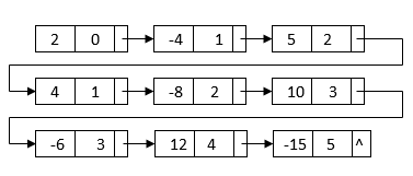
All of the terms we'll need to get the final outcome are in this linked list. The powers, on the other hand, do not sort it. It also has duplicate nodes with similar terms. We can merge sort the linked list depending on each node's power to get the final linked list:
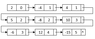
After sorting, the nodes with similar terms are clustered together. Then, for the final multiplication result, we can combine each set of like terms:

An algorithm can be used to describe these steps:

The first step in this approach is to multiply all term pairs from the two polynomials using a nested while loop. This takes O(nm) time to complete, where n and m are the number of terms in the two input polynomials, respectively. This procedure also produces a linked list with n times m nodes.
The linked list is then merged and sorted based on the power of each node. The time it takes to complete this process is O(nmlog (nm)).
We can use a two-pointer strategy to merge the like terms after sorting the linked list:

We utilize one pointer to create a like term group and another pointer to explore the like terms in the same group in this method. We add the coefficient of each like term we find to the start like term node. We change the start pointer to the next group and repeat the process to combine like terms once we finish one like term group. This method takes O(nm) time to complete since we need to visit n times m nodes.
Overall, the running time is O(nm) + O(nm\log (nm)) + O(nm) = O(nm\log (nm) ).
Code for Polynomial addition, subtraction and multiplication in C
#include<stdio.h>
#include<conio.h>
#include "poly.h"void main()
{
clrscr();
Polynomial *p1,*p2,*sum,*sub,*mul;
printf("\nENTER THE FIRST POLYNOMIAL.");
p1=createPolynomial();
printf("\nENTER THE SECOND POLYNOMIAL.");
p2=createPolynomial();
clrscr();
printf("\nFIRST : ");
displayPolynomial(p1);
printf("\nSECOND : ");
displayPolynomial(p2);
printf("\n\nADDITION IS : ");
sum=addPolynomial(p1,p2);
displayPolynomial(sum);
printf("\n\nSUBTRACTION IS : ");
sub=subPolynomial(p1,p2);
displayPolynomial(sub);
printf("\n\nMULTIPLICATION IS : ");
mul=mulPolynomial(p1,p2);
displayPolynomial(mul);
getch();
}
Key takeaway
- There may be times when you need to evaluate a large number of polynomial expressions and execute fundamental arithmetic operations on them, such as addition and subtraction.
- To multiply two polynomials, multiply the terms of one polynomial by the terms of the other polynomial.
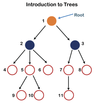
Fig 8: Tree
Each node in the above structure is labeled with a number. Each arrow in the diagram above represents a link between the two nodes.
Root - In a tree hierarchy, the root node is the highest node. To put it another way, the root node is the one that has no children. The root node of the tree is numbered 1 in the above structure. A parent-child relationship exists when one node is directly linked to another node.
Child node - If a node is a descendant of another node, it is referred to as a child node.
Parent - If a node has a sub-node, the parent of that sub-node is said to be that node.
Sibling - Sibling nodes are those that have the same parent.
Leaf node - A leaf node is a node in the tree that does not have any descendant nodes. A leaf node is the tree's bottommost node. In a generic tree, there can be any number of leaf nodes. External nodes are also known as leaf nodes.
Internal node - An internal node is a node that has at least one child node.
Ancestor node - Any previous node on a path from the root to that node is an ancestor of that node. There are no ancestors for the root node. Nodes 1, 2, and 5 are the ancestors of node 10 in the tree depicted above.
Descendant node - A descendant of a node is the direct successor of the supplied node. In the diagram above, node 10 is a descendent of node 5.
The tree data structure can be formed by using pointers to create the nodes dynamically. As shown below, the memory tree can be expressed as follows:
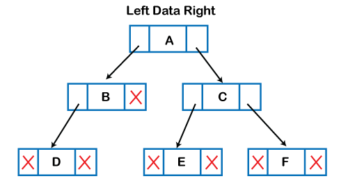
The memory representation of the tree data structure is shown in the diagram above. The node in the above structure has three fields. The data is stored in the second field, while the left child's address is stored in the first field and the right child's address is stored in the third field.
A node's structure can be defined as follows in programming:
Struct node
{
int data;
Struct node *left;
Struct node *right;
}
Because binary trees can only have two offspring, and generic trees can have more than two, the above structure can only be defined for binary trees. In comparison to the binary tree, the structure of the node in generic trees would be different.
Traversal is a process to visit all the nodes of a tree and may print their values too. Because all nodes are connected via edges (links) we always start from the root (head) node. That is, we cannot randomly access a node in a tree. There are three ways which we use to traverse a tree −
● In-order Traversal
● Pre-order Traversal
● Post-order Traversal
Generally, we traverse a tree to search or locate a given item or key in the tree or to print all the values it contains.
In-order Traversal
In this traversal method, the left subtree is visited first, then the root and later the right subtree. We should always remember that every node may represent a subtree itself.
If a binary tree is traversed in-order, the output will produce sorted key values in an ascending order.
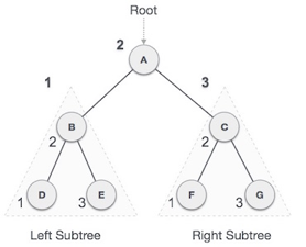
Fig 9: Inorder
We start from A, and following in-order traversal, we move to its left subtree B. B is also traversed in-order. The process goes on until all the nodes are visited. The output of inorder traversal of this tree will be −
D → B → E → A → F → C → G
Algorithm
Until all nodes are traversed −
Step 1 − Recursively traverse left subtree.
Step 2 − Visit root node.
Step 3 − Recursively traverse right subtree.
Pre-order Traversal
In this traversal method, the root node is visited first, then the left subtree and finally the right subtree.
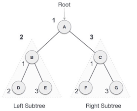
Fig 10: Pre order
We start from A, and following pre-order traversal, we first visit A itself and then move to its left subtree B. B is also traversed pre-order. The process goes on until all the nodes are visited. The output of pre-order traversal of this tree will be −
A → B → D → E → C → F → G
Algorithm
Until all nodes are traversed −
Step 1 − Visit root node.
Step 2 − Recursively traverse left subtree.
Step 3 − Recursively traverse right subtree.
Post-order Traversal
In this traversal method, the root node is visited last, hence the name. First we traverse the left subtree, then the right subtree and finally the root node.
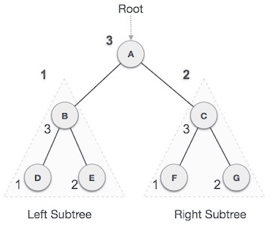
Fig 11: Post order
We start from A, and following Post-order traversal, we first visit the left subtree B. B is also traversed post-order. The process goes on until all the nodes are visited. The output of post-order traversal of this tree will be −
D → E → B → F → G → C → A
Algorithm
Until all nodes are traversed −
Step 1 − Recursively traverse left subtree.
Step 2 − Recursively traverse right subtree.
Step 3 − Visit root node.
The Binary tree means that the node can have a maximum of two children. Here, the binary name itself suggests 'two'; therefore, each node can have either 0, 1 or 2 children.
Let's understand the binary tree through an example.
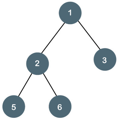
Fig 12: Example
The above tree is a binary tree because each node contains the utmost two children. The logical representation of the above tree is given below:
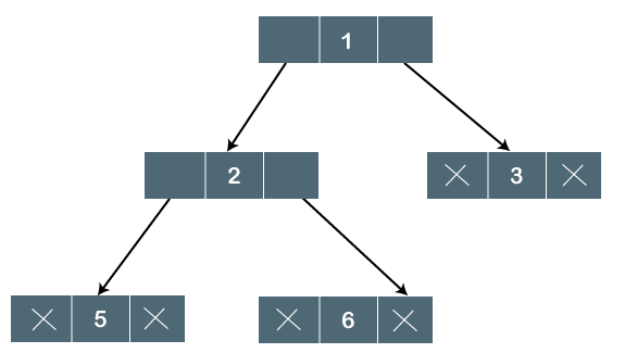
Fig 13: Logical representation
In the above tree, node 1 contains two pointers, i.e., left and a right pointer pointing to the left and right node respectively. The node 2 contains both the nodes (left and right node); therefore, it has two pointers (left and right). The nodes 3, 5 and 6 are the leaf nodes, so all these nodes contain NULL pointer on both left and right parts.
Properties of Binary Tree
● At each level of i, the maximum number of nodes is 2i.
● The height of the tree is defined as the longest path from the root node to the leaf node. The tree which is shown above has a height equal to 3. Therefore, the maximum number of nodes at height 3 is equal to (1+2+4+8) = 15. In general, the maximum number of nodes possible at height h is (20 + 21 + 22+….2h) = 2h+1 -1.
● The minimum number of nodes possible at height h is equal to h+1.
● If the number of nodes is minimum, then the height of the tree would be maximum. Conversely, if the number of nodes is maximum, then the height of the tree would be minimum.
If there are 'n' number of nodes in the binary tree.
The minimum height can be computed as:
As we know that,
n = 2h+1 -1
n+1 = 2h+1
Taking log on both the sides,
Log2(n+1) = log2(2h+1)
Log2(n+1) = h+1
h = log2(n+1) - 1
The maximum height can be computed as:
As we know that,
n = h+1
h= n-1
Types of Binary Tree
There are four types of Binary tree:
● Full/ proper/ strict Binary tree
● Complete Binary tree
● Perfect Binary tree
● Degenerate Binary tree
● Balanced Binary tree
Key takeaway
- The Binary tree means that the node can have a maximum of two children. Here, binary name itself suggests 'two'; therefore, each node can have either 0, 1 or 2 children.
A binary search tree is a type of binary tree in which the nodes are organized in a predetermined sequence. This is referred to as an ordered binary tree.
The value of all nodes in the left sub-tree is less than the value of the root in a binary search tree. Similarly, the value of all nodes in the right subtree is larger than or equal to the root's value. This rule will be applied recursively to all of the root's left and right subtrees.
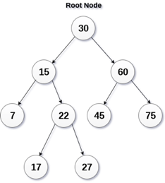
Fig 14: Binary search tree
A Binary Search Tree (BST) is a tree in which all nodes have the properties listed below.
● The key of the left subtree has a lower value than the key of its parent (root) node.
● The value of the right subkey tree's is larger than or equal to the value of the key of its parent (root) node.
● As a result, BST separates all of its sub-trees into two segments: the left and right subtrees, and can be characterized as
Left_subtree (keys) < node (key) ≤ right_subtree (keys)
Insertion
The insertion operation in a binary search tree takes O(log n) time to complete. A new node is always added as a leaf node in a binary search tree. The following is how the insertion procedure is carried out...
Step 1: Create a newNode with the specified value and NULL left and right.
Step 2: Make sure the tree isn't empty.
Step 3 - Set root to newNode if the tree is empty.
Step 4 - If the tree isn't empty, see if newNode's value is smaller or larger than the node's value (here it is root node).
Step 5 - Go to the node's left child if newNode is smaller or equal to it. Move to new Nodes right child if the newNode is larger than the node.
Step 6- Continue in this manner until we reach the leaf node (i.e., reaches to NULL).
Step 7 - Once you've reached the leaf node, insert the newNode as a left child if it's smaller or equal to the leaf node, or as a right child otherwise.
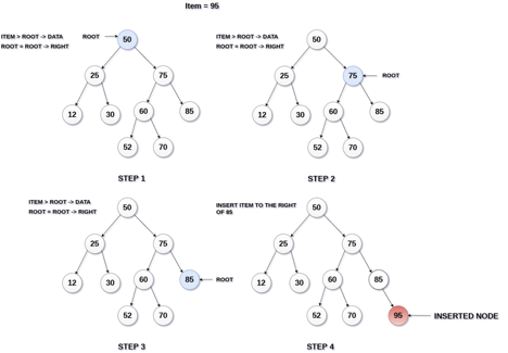
Fig 15: Example of insertion
Deletion
The deletion process in a binary search tree takes O(log n) time to complete. The three scenarios for removing a node from a Binary search tree are as follows...
Case 1: Deleting a Leaf node (A node with no children)
Case 2: Deleting a node with one child
Case 3: Deleting a node with two children
Case 1: Deleting a Leaf node
To delete a leaf node from BST, follow these steps...
Step 1: Using the search function, locate the node to be eliminated.
Step 2 - If the node is a leaf, delete it with the free function and end the function.
Case 2: Deleting a node with one child
To delete a node with one child from BST, we utilize the procedures below...
Step 1: Using the search function, locate the node to be eliminated.
Step 2 - Create a link between the parent node and the child node if it only has one child.
Step 3: Using the free function, delete the node and exit the function
Case 3: Deleting a node with two children
To delete a node with two children from BST, we utilize the procedures below...
Step 1: Using the search function, locate the node to be eliminated.
Step 2 - Find the largest node in the left subtree (OR the smallest node in the right subtree) if it has two children.
Step 3 - Swap the deleting node with the node discovered in the previous step.
Step 4 - Next, see if deleting the node resulted in case 1 or case 2, if not, move to step 2.
Step 5 - If case 1 applies, delete it using case 1 reasoning.
Step 6- If case 2 applies, delete it using case 2 reasoning.
Step 7 - Continue in this manner until the node has been removed from the tree.
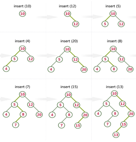
Example
Create a Binary Search Tree by adding the integers in the following order…
10,12,5,4,20,8,7,15 and 13
The following items are added into a Binary Search Tree in the following order...
Key takeaway
A binary search tree is a type of binary tree in which the nodes are organized in a predetermined sequence.
This is referred to as an ordered binary tree.
Expression trees are one of the most effective methods for representing language-level code as data stored in a tree-like structure. An expression tree is a representation of a lambda expression in memory. The tree clarifies and transparentes the structure holding the lambda expression. The expression tree was designed to turn code into strings that may be supplied as inputs to other processes. It contains the query's actual elements, rather than the query's actual result.
One of the most essential characteristics of expression trees is that they are immutable, which means that altering an existing expression tree requires creating a new expression tree by copying and updating the existing tree expression. In programming, an expression tree is commonly constructed using postfix expressions, which read one symbol at a time. A one-node tree is formed and a pointer to it is pushed into a stack if the symbol is an operand.
The expression tree is a type of tree that is used to represent different types of expressions. The expressional assertions are represented using a tree data structure. The operators are always represented by the internal node in this tree.
● The operands are always denoted by the leaf nodes.
● These operands are always used in the operations.
● The operator in the deepest part of the tree is always given priority.
● The operator who is not very deep in the tree is always given the lowest priority compared to the operators who are very deep in the tree.
● The operand will always be present at a depth of the tree, making it the most important of all the operators.
● In summary, as compared to the other operators at the top of the tree, the value existing at a depth of the tree has the most importance.
● These expression trees are primarily used to assess, analyse, and modify a variety of expressions.
● It's also utilised to determine each operator's associativity in the phrase.
● The + operator, for example, is left-associative, while the / operator is right-associative.
● Using expression trees, the conundrum of this associativity has been solved.
● A context-free grammar is used to create these expression trees.
● In context-free grammars, we've put a rule in front of each grammar production.
● These rules are also known as semantic rules, and we can easily design expression trees using these semantic rules.
● It is part of the semantic analysis process and is one of the most important aspects of compiler design.
● We will employ syntax-directed translations in our semantic analysis, and we will create an annotated parse tree as output.
● The basic parse associated with the type property and each production rule makes up an annotated parse tree.
● The fundamental goal of using expression trees is to create complex expressions that can be easily evaluated using these trees.
● It's immutable, which means that once we've generated an expression tree, we can't change or modify it.
● It is necessary to completely construct the new expression tree in order to make more changes.
● It's also used to evaluate expressions with postfixes, prefixes, and infixes.
Expression trees are extremely useful for encoding language-level code in the form of data, which is mostly kept in a tree-like structure. It's also used in the lambda expression's memory representation. We can represent the lambda expression more openly and explicitly using the tree data structure. It is first constructed to transform the code segment to the data segment, allowing the expression to be evaluated quickly.
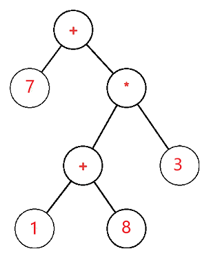
The expression tree is a binary tree in which the operand is represented by the exterior or leaf node and the operators are represented by the internal or parent node. For example, the expression tree for 7 + ((1+8)*3) would be:
Use of Expression tree
● The fundamental goal of using expression trees is to create complex expressions that can be easily evaluated using these trees.
● It's also used to determine each operator's associativity in the phrase.
● It's also used to evaluate expressions with postfixes, prefixes, and infixes.
AVL Tree was invented by GM Adelson - Velsky and EM Landis in 1962. The tree is named AVL in honor of its inventors.
AVL Tree can be defined as a height balanced binary search tree in which each node is associated with a balance factor which is calculated by subtracting the height of its right subtree from that of its left sub-tree.
Tree is said to be balanced if the balance factor of each node is in between -1 to 1, otherwise, the tree will be unbalanced and need to be balanced.
Balance Factor (k) = height (left(k)) - height (right(k))
If balance factor of any node is 1, it means that the left sub-tree is one level higher than the right subtree.
If balance factor of any node is 0, it means that the left subtree and right subtree contain equal height.
If balance factor of any node is -1, it means that the left sub-tree is one level lower than the right subtree.
An AVL tree is given in the following figure. We can see that, balance factor associated with each node is in between -1 and +1. Therefore, it is an example of AVL tree.
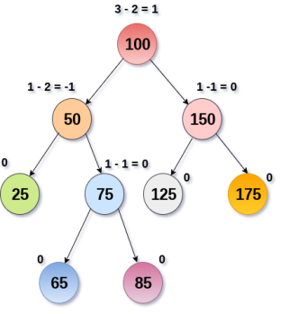
Fig 16 – AVL Tree
Complexity
Algorithm | Average case | Worst case |
Space | o(n) | o(n) |
Search | o(log n) | o(log n) |
Insert | o(log n) | o(log n) |
Delete | o(log n) | o(log n) |
Operations on AVL tree
Due to the fact that, AVL tree is also a binary search tree therefore, all the operations are performed in the same way as they are performed in a binary search tree. Searching and traversing do not lead to the violation in property of AVL tree. However, insertion and deletion are the operations which can violate this property and therefore, they need to be revisited.
SN | Operation | Description |
1 | Insertion | Insertion in AVL tree is performed in the same way as it is performed in a binary search tree. However, it may lead to violation in the AVL tree property and therefore the tree may need balancing. The tree can be balanced by applying rotations. |
2 | Deletion | Deletion can also be performed in the same way as it is performed in a binary search tree. Deletion may also disturb the balance of the tree therefore, various types of rotations are used to rebalance the tree. |
Why AVL Tree?
AVL tree controls the height of the binary search tree by not letting it to be skewed. The time taken for all operations in a binary search tree of height h is O(h). However, it can be extended to O(n) if the BST becomes skewed (i.e. worst case). By limiting this height to log n, AVL tree imposes an upper bound on each operation to be O(log n) where n is the number of nodes.
AVL Rotations
We perform rotation in AVL tree only in case if Balance Factor is other than -1, 0, and 1. There are basically four types of rotations which are as follows:
- L L rotation: Inserted node is in the left subtree of left subtree of A
- R R rotation: Inserted node is in the right subtree of right subtree of A
- L R rotation: Inserted node is in the right subtree of left subtree of A
- R L rotation: Inserted node is in the left subtree of right subtree of A
Where node A is the node whose balance Factor is other than -1, 0, 1.
The first two rotations LL and RR are single rotations and the next two rotations LR and RL are double rotations. For a tree to be unbalanced, minimum height must be at least 2, Let us understand each rotation
1. RR Rotation
When BST becomes unbalanced, due to a node is inserted into the right subtree of the right subtree of A, then we perform RR rotation, RR rotation is an anticlockwise rotation, which is applied on the edge below a node having balance factor -2
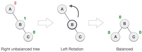
In above example, node A has balance factor -2 because a node C is inserted in the right subtree of A right subtree. We perform the RR rotation on the edge below A.
2. LL Rotation
When BST becomes unbalanced, due to a node is inserted into the left subtree of the left subtree of C, then we perform LL rotation, LL rotation is clockwise rotation, which is applied on the edge below a node having balance factor 2.
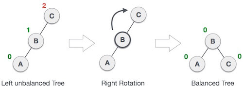
In above example, node C has balance factor 2 because a node A is inserted in the left subtree of C left subtree. We perform the LL rotation on the edge below A.
3. LR Rotation
Double rotations are bit tougher than single rotation which has already explained above. LR rotation = RR rotation + LL rotation, i.e., first RR rotation is performed on subtree and then LL rotation is performed on full tree, by full tree we mean the first node from the path of inserted node whose balance factor is other than -1, 0, or 1.
Let us understand each and every step very clearly:
State | Action |
 | A node B has been inserted into the right subtree of A the left subtree of C, because of which C has become an unbalanced node having balance factor 2. This case is L R rotation where: Inserted node is in the right subtree of left subtree of C |
 | As LR rotation = RR + LL rotation, hence RR (anticlockwise) on subtree rooted at A is performed first. By doing RR rotation, node A, has become the left subtree of B. |
 | After performing RR rotation, node C is still unbalanced, i.e., having balance factor 2, as inserted node A is in the left of left of C |
 | Now we perform LL clockwise rotation on full tree, i.e. on node C. Node C has now become the right subtree of node B, A is left subtree of B |
 | Balance factor of each node is now either -1, 0, or 1, i.e. BST is balanced now. |
4. RL Rotation
As already discussed, that double rotations are bit tougher than single rotation which has already explained above. R L rotation = LL rotation + RR rotation, i.e., first LL rotation is performed on subtree and then RR rotation is performed on full tree, by full tree we mean the first node from the path of inserted node whose balance factor is other than -1, 0, or 1.
State | Action |
 | A node B has been inserted into the left subtree of C the right subtree of A, because of which A has become an unbalanced node having balance factor - 2. This case is RL rotation where: Inserted node is in the left subtree of right subtree of A |
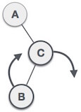 | As RL rotation = LL rotation + RR rotation, hence, LL (clockwise) on subtree rooted at C is performed first. By doing RR rotation, node C has become the right subtree of B. |
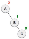 | After performing LL rotation, node A is still unbalanced, i.e. having balance factor -2, which is because of the right-subtree of the right-subtree node A. |
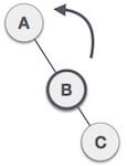 | Now we perform RR rotation (anticlockwise rotation) on full tree, i.e. on node A. Node C has now become the right subtree of node B, and node A has become the left subtree of B. |
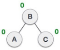 | Balance factor of each node is now either -1, 0, or 1, i.e., BST is balanced now. |
Q: Construct an AVL tree having the following elements
H, I, J, B, A, E, C, F, D, G, K, L
1. Insert H, I, J
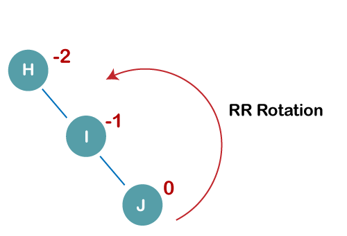
On inserting the above elements, especially in the case of H, the BST becomes unbalanced as the Balance Factor of H is -2. Since the BST is right-skewed, we will perform RR Rotation on node H.
The resultant balance tree is:
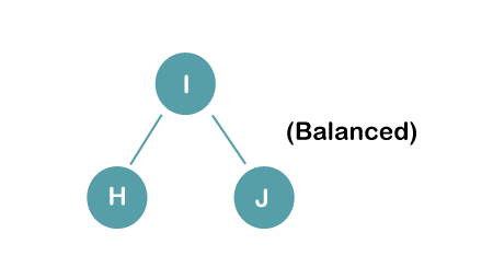
2. Insert B, A
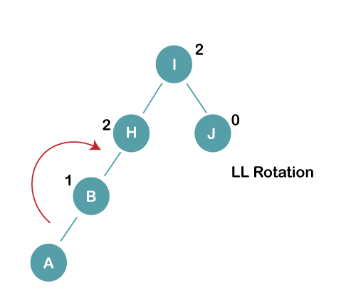
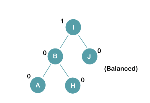
On inserting the above elements, especially in case of A, the BST becomes unbalanced as the Balance Factor of H and I is 2, we consider the first node from the last inserted node i.e. H. Since the BST from H is left-skewed, we will perform LL Rotation on node H.
The resultant balance tree is:
3. Insert E
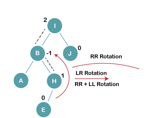
On inserting E, BST becomes unbalanced as the Balance Factor of I is 2, since if we travel from E to I we find that it is inserted in the left subtree of right subtree of I, we will perform LR Rotation on node I. LR = RR + LL rotation
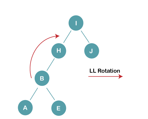
3 a) We first perform RR rotation on node B
The resultant tree after RR rotation is:
3b) We first perform LL rotation on the node I
The resultant balanced tree after LL rotation is:
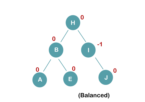
4. Insert C, F, D
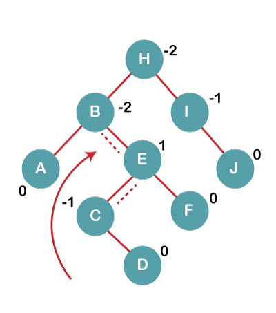
On inserting C, F, D, BST becomes unbalanced as the Balance Factor of B and H is -2, since if we travel from D to B we find that it is inserted in the right subtree of left subtree of B, we will perform RL Rotation on node I. RL = LL + RR rotation.
4a) We first perform LL rotation on node E
The resultant tree after LL rotation is:
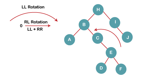
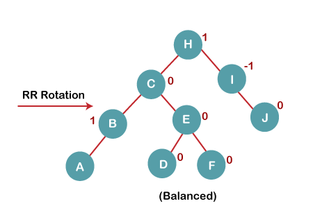
4b) We then perform RR rotation on node B
The resultant balanced tree after RR rotation is:
5. Insert G
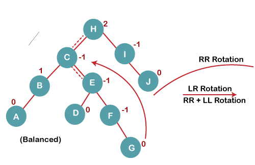
On inserting G, BST become unbalanced as the Balance Factor of H is 2, since if we travel from G to H, we find that it is inserted in the left subtree of right subtree of H, we will perform LR Rotation on node I. LR = RR + LL rotation.
5 a) We first perform RR rotation on node C
The resultant tree after RR rotation is:
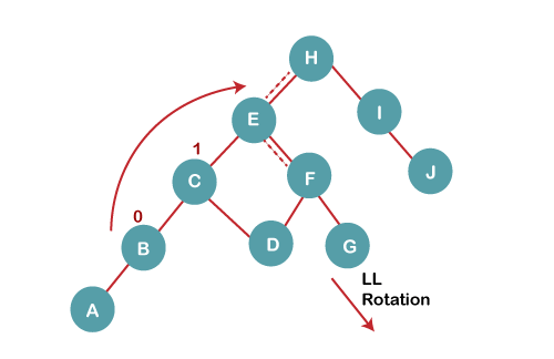
5 b) We then perform LL rotation on node H
The resultant balanced tree after LL rotation is:
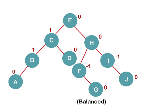
6. Insert K
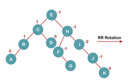
On inserting K, BST becomes unbalanced as the Balance Factor of I is -2. Since the BST is right-skewed from I to K, hence we will perform RR Rotation on the node I.
The resultant balanced tree after RR rotation is:
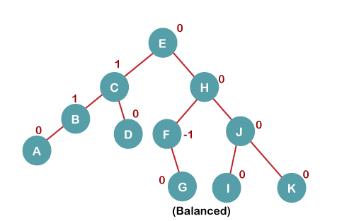
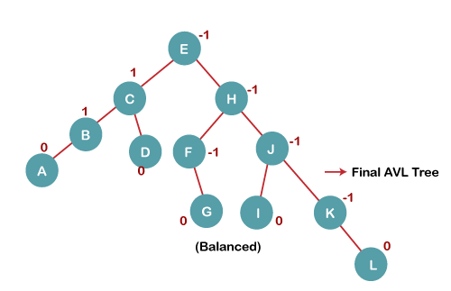
7. Insert L
On inserting the L tree is still balanced as the Balance Factor of each node is now either, -1, 0, +1. Hence the tree is a Balanced AVL tree
Key takeaway
- AVL Tree was invented by GM Adelson - Velsky and EM Landis in 1962. The tree is named AVL in honor of its inventors.
- AVL Tree can be defined as a height balanced binary search tree in which each node is associated with a balance factor which is calculated by subtracting the height of its right subtree from that of its left sub-tree.
- Tree is said to be balanced if the balance factor of each node is in between -1 to 1, otherwise, the tree will be unbalanced and need to be balanced.
A binary heap is a data structure that resembles a complete binary tree in appearance. The ordering features of the heap data structure are explained here. A Heap is often represented by an array. We'll use H to represent a heap.
Because the elements of a heap are kept in an array, the position of the parent node of the ith element can be located at i/2 if the starting index is 1. Position 2i and 2i + 1 are the left and right children of the ith node, respectively.
Based on the ordering property, a binary heap can be classed as a max-heap or a min-heap.
Max Heap
A node's key value is larger than or equal to the key value of the highest child in this heap.
Hence, H[Parent(i)] ≥ H[i]
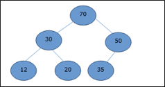
Fig 17: max heap
Max Heap Construction Algorithm
The technique for creating Min Heap is similar to that for creating Max Heap, only we use min values instead of max values.
By inserting one element at a time, we will derive a method for max heap. The property of a heap must be maintained at all times. We also presume that we are inserting a node into an already heapify tree while inserting.
● Step 1: Make a new node at the bottom of the heap.
● Step 2: Give the node a new value.
● Step 3: Compare this child node's value to that of its parent.
● Step 4: If the parent's value is smaller than the child's, swap them.
● Step 5: Repeat steps 3 and 4 until the Heap property is maintained.
Min Heap
In mean-heap, a node's key value is less than or equal to the lowest child's key value.
Hence, H[Parent(i)] ≤ H[i]
Basic operations with respect to Max-Heap are shown below in this context. The insertion and deletion of elements in and out of heaps necessitates element reordering. As a result, the Heapify function must be used.
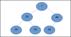
Fig 18: Min heap
Max Heap Deletion Algorithm
Let's create an algorithm for deleting from the maximum heap. The root of the Max (or Min) Heap is always deleted to remove the maximum (or minimum) value.
● Step 1: Remove the root node first.
● Step 2: Move the last element from the previous level to the root.
● Step 3: Compare this child node's value to that of its parent.
● Step 4: If the parent's value is smaller than the child's, swap them.
● Step 5: Repeat steps 3 and 4 until the Heap property is maintained.
Key takeaway
The ordering features of the heap data structure are explained here. A Heap is often represented by an array.
References:
- Fundamentals of Computer Algorithms by Horowitz, Sahni,Galgotia Pub. 2001 ed.
- Data Structures using C and C++ by Y. Langsam, Pearson Education.
- Data Structures using C by Tanenbaum, Pearson Education
- Introduction to Algorithms, by Thomas Corman III edition, PHI
- Analysis and Design of Algorithms: A Beginner's Approach, by Rajesh K. Shukla, Willey Publications
- Data Structures: A Pseudocode Approach with C by Richard F. Gilberg and Behrouz Forouzan.