Unit - 5
Algorithms
Advanced data structures are one of the most important areas of data science since they are used to store, organize, and manage data and information in order to make it more efficient, accessible, and modifiable. They serve as the foundation for creating efficient and successful software and algorithms. Being a skilled programmer necessitates knowing how to develop and construct a good data structure. Its scope is also expanding as new information technology and working techniques emerge.
Many algorithms' efficiency and performance are directly proportional to the data they use to perform calculations and other data operations. Data structures perform the basic function of keeping data in main memory during run-time or programme execution, hence memory management is particularly significant since it has a direct impact on the space complexity of a programme or algorithm. As a result, selecting a suitable data structure is critical to programme efficiency and performance.
List of Advanced Data Structures
Advanced-Data structures have multiplied into a plethora of manifolds. The following are the broad categories into which sophisticated data structures are classified:
● Primitive types
● Composite or non-primitive type
● Abstract data types
● Linear Data Structures
● Tree types
● Hash-based structures
● Graphs
It is a greedy algorithm that solves the single-source shortest path problem for a directed graph G = (V, E) with nonnegative edge weights, i.e., w (u, v) ≥ 0 for each edge (u, v) ∈ E.
Dijkstra's Algorithm maintains a set S of vertices whose final shortest - path weights from the source s have already been determined. That's for all vertices v ∈ S; we have d [v] = δ (s, v). The algorithm repeatedly selects the vertex u ∈ V - S with the minimum shortest - path estimate, insert u into S and relaxes all edges leaving u.
Because it always chooses the "lightest" or "closest" vertex in V - S to insert into set S, it is called as the greedy strategy.
Dijkstra's Algorithm (G, w, s)
1. INITIALIZE - SINGLE - SOURCE (G, s)
2. S←∅
3. Q←V [G]
4. While Q ≠ ∅
5. Do u ← EXTRACT - MIN (Q)
6. S ← S ∪ {u}
7. For each vertex v ∈ Adj [u]
8. Do RELAX (u, v, w)
Analysis: The running time of Dijkstra's algorithm on a graph with edges E and vertices V can be expressed as a function of |E| and |V| using the Big - O notation. The simplest implementation of the Dijkstra's algorithm stores vertices of set Q in an ordinary linked list or array, and operation Extract - Min (Q) is simply a linear search through all vertices in Q. In this case, the running time is O (|V2 |+|E|=O(V2 ).
Example:

Solution:
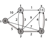
Step1: Q =[s, t, x, y, z]
We scanned vertices one by one and find out its adjacent. Calculate the distance of each adjacent to the source vertices.
We make a stack, which contains those vertices which are selected after computation of shortest distance.
Firstly we take's' in stack M (which is a source)
- M = [S] Q = [t, x, y, z]
Step 2: Now find the adjacent of s that are t and y.
- Adj [s] → t, y [Here s is u and t and y are v]

Case - (i) s → t
d [v] > d [u] + w [u, v]
d [t] > d [s] + w [s, t]
∞ > 0 + 10 [false condition]
Then d [t] ← 10
π [t] ← 5
Adj [s] ← t, y
Case - (ii) s→ y
d [v] > d [u] + w [u, v]
d [y] > d [s] + w [s, y]
∞ > 0 + 5 [false condition]
∞ > 5
Then d [y] ← 5
π [y] ← 5
By comparing case (i) and case (ii)
Adj [s] → t = 10, y = 5
y is shortest
y is assigned in 5 = [s, y]
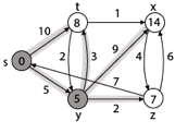
Step 3: Now find the adjacent of y that is t, x, z.
- Adj [y] → t, x, z [Here y is u and t, x, z are v]
Case - (i) y →t
d [v] > d [u] + w [u, v]
d [t] > d [y] + w [y, t]
10 > 5 + 3
10 > 8
Then d [t] ← 8
π [t] ← y
Case - (ii) y → x
d [v] > d [u] + w [u, v]
d [x] > d [y] + w [y, x]
∞ > 5 + 9
∞ > 14
Then d [x] ← 14
π [x] ← 14
Case - (iii) y → z
d [v] > d [u] + w [u, v]
d [z] > d [y] + w [y, z]
∞ > 5 + 2
∞ > 7
Then d [z] ← 7
π [z] ← y
By comparing case (i), case (ii) and case (iii)
Adj [y] → x = 14, t = 8, z =7
z is shortest
z is assigned in 7 = [s, z]

Step - 4 Now we will find adj [z] that are s, x
- Adj [z] → [x, s] [Here z is u and s and x are v]
Case - (i) z → x
d [v] > d [u] + w [u, v]
d [x] > d [z] + w [z, x]
14 > 7 + 6
14 > 13
Then d [x] ← 13
π [x] ← z
Case - (ii) z → s
d [v] > d [u] + w [u, v]
d [s] > d [z] + w [z, s]
0 > 7 + 7
0 > 14
∴ This condition does not satisfy so it will be discarded.
Now we have x = 13.

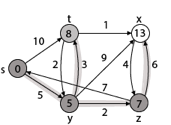
Step 5: Now we will find Adj [t]
Adj [t] → [x, y] [Here t is u and x and y are v]
Case - (i) t → x
d [v] > d [u] + w [u, v]
d [x] > d [t] + w [t, x]
13 > 8 + 1
13 > 9
Then d [x] ← 9
π [x] ← t
Case - (ii) t → y
d [v] > d [u] + w [u, v]
d [y] > d [t] + w [t, y]
5 > 10
∴ This condition does not satisfy so it will be discarded.

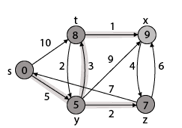
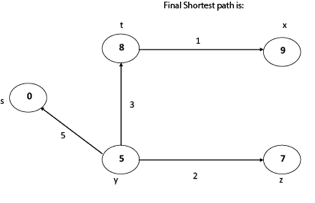
Thus, we get all shortest path vertex as
Weight from s to y is 5
Weight from s to z is 7
Weight from s to t is 8
Weight from s to x is 9
These are the shortest distance from the source's' in the given graph.

Disadvantage of Dijkstra's Algorithm:
- It does a blind search, so wastes a lot of time while processing.
- It can't handle negative edges.
- It leads to the acyclic graph and most often cannot obtain the right shortest path.
- We need to keep track of vertices that have been visited.
In Dijkstra’s algorithm, two sets are maintained, one set contains list of vertices already included in SPT (Shortest Path Tree), other set contains vertices not yet included. With adjacency list representation, all vertices of a graph can be traversed in O(V+E) time using BFS. The idea is to traverse all vertices of graph using BFS and use a Min Heap to store the vertices not yet included in SPT (or the vertices for which shortest distance is not finalized yet).
Min Heap is used as a priority queue to get the minimum distance vertex from set of not yet included vertices. Time complexity of operations like extract-min and decrease-key value is O(LogV) for Min Heap.
Following are the detailed steps.
1) Create a Min Heap of size V where V is the number of vertices in the given graph. Every node of min heap contains vertex number and distance value of the vertex.
2) Initialize Min Heap with source vertex as root (the distance value assigned to source vertex is 0). The distance value assigned to all other vertices is INF (infinite).
3) While Min Heap is not empty, do following
a) Extract the vertex with minimum distance value node from Min Heap. Let the extracted vertex be u.
b) For every adjacent vertex v of u, check if v is in Min Heap. If v is in Min Heap and distance value is more than weight of u-v plus distance value of u, then update the distance value of v.
Let us understand with the following example. Let the given source vertex be 0
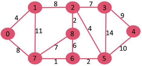
Initially, distance value of source vertex is 0 and INF (infinite) for all other vertices. So source vertex is extracted from Min Heap and distance values of vertices adjacent to 0 (1 and 7) are updated. Min Heap contains all vertices except vertex 0.
The vertices in green color are the vertices for which minimum distances are finalized and are not in Min Heap

Since distance value of vertex 1 is minimum among all nodes in Min Heap, it is extracted from Min Heap and distance values of vertices adjacent to 1 are updated (distance is updated if the vertex is in Min Heap and distance through 1 is shorter than the previous distance). Min Heap contains all vertices except vertex 0 and 1.

Pick the vertex with minimum distance value from min heap. Vertex 7 is picked. So min heap now contains all vertices except 0, 1 and 7. Update the distance values of adjacent vertices of 7. The distance value of vertex 6 and 8 becomes finite (15 and 9 respectively).

Pick the vertex with minimum distance from min heap. Vertex 6 is picked. So min heap now contains all vertices except 0, 1, 7 and 6. Update the distance values of adjacent vertices of 6. The distance value of vertex 5 and 8 are updated.

Above steps are repeated till min heap doesn’t become empty. Finally, we get the following shortest path tree.

Key takeaway
- Warshall’s algorithm constructs transitive closure of a given directed graph.
- In directed graphs there are n vertices.
- A graph with each edge directed is called a directed OR digraph graph.
- Dijkstra’s algorithm is the iterative algorithmic process to provide us with the shortest path from one specific starting node to all other nodes of a graph.
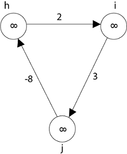
It's a weighted graph in which each edge's total weight is negative. A chain is formed when a graph has a negative edge. If the output is negative after performing the chain, the weight and condition will be eliminated. We can't have the shortest path in it if the weight is smaller than negative and -.
In a nutshell, if the output is -ve, both conditions are ignored.
● - ∞
● Not less than 0
We can't have the shortest Path, either.
Example
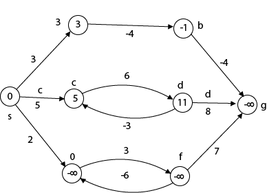
Beginning from s
Adj [s] = [a, c, e]
Weight from s to a is 3
Let's say we want to find a path from s→c. As a result, we have two path /weight.
s to c = 5, s→c→d→c=8
But s→c is minimum
So s→c = 5
Let's say we want to find a path from s→e. So we're back to having two options.
s→e = 2, s→e→f→e=-1
As -1 < 0 ∴ Condition gets discarded. If we execute this chain, we will get - ∞. So we can't get the shortest path ∴ e = ∞.

The effects of negative weights and the negative weight cycle on the shortest path weights are shown in this diagram.
Because there is only one path from "s to a" (the path <s, a>), δ (s, a) = w (s, a) = 3.
Furthermore, there is only one path from "s to b", so δ (s, b) = w (s, a) + w (a, b) = 3 + (-4) = - 1.
There are an unlimited number of paths from "s to c": <s, c, d, c>, <s, c, d, c, d, c>, and so on. Because the cycle <c, d, c> has a weight of δ(c, d) = w (c, d) + w (d, c) = 6 + (-3) = 3, the shortest path from s to c is s, c>, which has a weight of δ(s, c) = 5.
Similarly, the shortest path from "s to d" is with weight δ (s, d) = w (s, c) + w (s, d) = 11.
Weight (s, d) = w (s, c) + w (s, d) = 11 is also the shortest path from "s to d."
Similarly, there exist an endless number of pathways from s to e:,, and so on. Since the cycle has weight δ (e, f) = w (e, f) + w (f, e) = 3 + (-6) = -3. So - 3 < 0, However, there is no shortest path from s to e, therefore - 3 0. B8y is in the midst of a negative weight cycle. As a result, the path from s to e has arbitrary big negative weights, and δ (s, e) = - ∞.
In the same way, δ (s, f) = - ∞ Because g can be reached via f, we can also find a path from s to g with any large negative weight, and δ (s, g) = - ∞

Negative weight cycle also affects vertices h, I and g. They are also inaccessible from the source node, resulting in a distance of - ∞ to three nodes from the source (h, i, j).
If there are no cycles in a graph, it is called an acyclic graph, and an acyclic graph is the polar opposite of a cyclic graph.
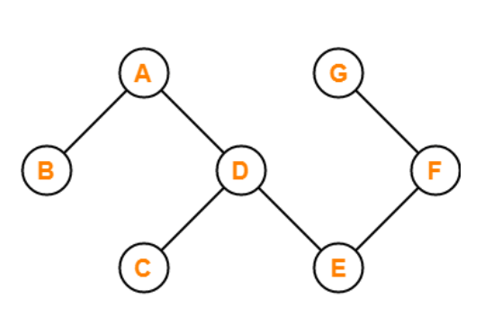
The graph in the preceding figure is acyclic because it has no cycles. That is, if we start from vertex B and tour the graph, there is no single path that will traverse all of the vertices and terminate at the same vertex, which is vertex B.
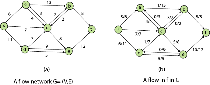
The following is the most obvious flow network issue:
Problem1: The maximum flow problem aims to discover a flow with the highest value given a flow network G = (V, E).
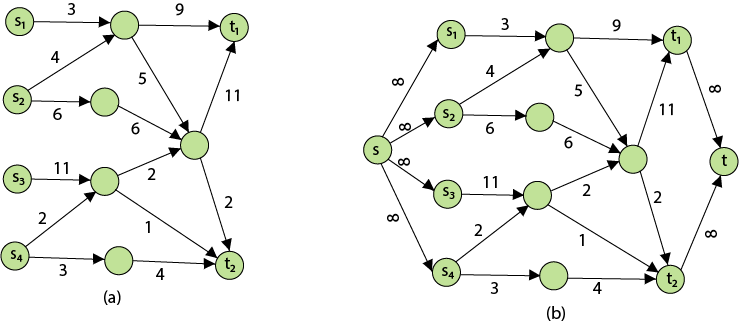
Problem 2: The maximum flow problem with numerous sources and sinks is similar to the maximum flow problem with a set of {s1,s2,s3.......sn} sources and a set of {t1,t2,t3.......tn} sinks.
Thankfully, this issue isn't as serious as normal maximum flow. We define a new flow network G' by adding additional sources and sinks to the flow network G.
● A super source s,
● A super sink t,
● For each si, add edge (s, si) with capacity ∞, and
● For each ti,add edge (ti,t) with capacity ∞
Figure depicts a flow network with numerous sources and sinks, as well as an analogous single source and sink flow network.

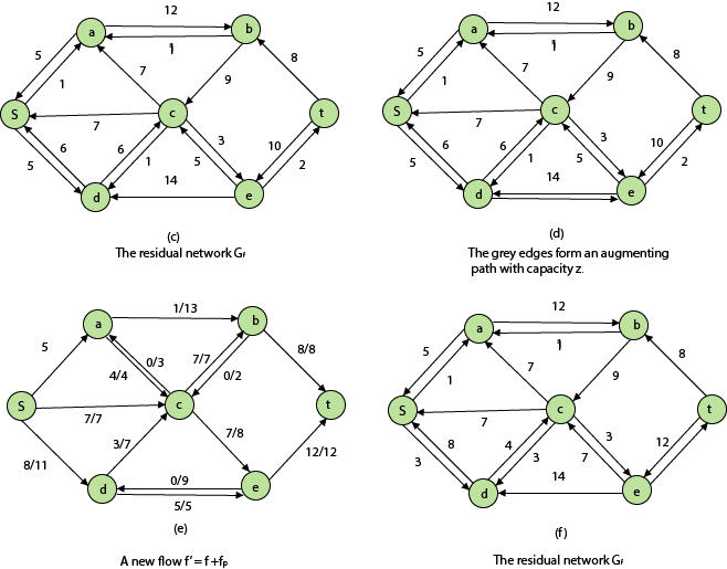
Residual Networks: The Residual Network is made out of a network edge that can accept extra traffic. Assume we have a G = (V, E) flow network with source s and sink t. Examine a pair of vertices u, v ∈ V, and consider f as a flow in G. The residual capacity of (u, v) is the sum of additional net flow we may push from u to v before exceeding the capacity c (u, v).

The residual capacity cf (u,v) is greater than the capacity c when the net flow f (u, v) is negative (u, v).
For Example: if c (u, v) = 16 and f (u, v) =16 and f (u, v) = -4, then the residual capacity cf (u,v) is 20.
Given a flow network G = (V, E) and a flow f, the residual network of G induced by f is Gf = (V, Ef), where

That is, each residual network edge, or residual edge, can permit a net flow that is strictly positive.
Augmenting Path: An augmenting path p is a simple path from s to t in the residual network Gf given a flow network G = (V, E) and a flow f. The residual network approach allows each augmenting path edge (u, v) to accept some additional positive net flow from u to v without violating the edge's capacity constraint.
Let G = (V, E) be a flow network with flow f. The residual capacity of an augmenting path p is

The maximum amount of flow that may be pushed through the augmenting channel is known as the residual capacity. If an augmenting path exists, each of its edges has a positive capacity. This fact will be used to calculate the maximum flow in a flow network.


It is a Dynamic Programming method in which the previous output is used as the input for the next.
Chain denotes that one matrix's column is always equal to the second matrix's row.
Find the most efficient technique to multiply these matrices together given a sequence of matrices. The issue is not so much with performing the multiplications as it is with deciding which sequence to conduct them in.
Because matrix multiplication is associative, we have a lot of alternatives when multiplying a chain of matrices. In other words, the result will be the same regardless of how we parenthesize the product.
For four matrices A, B, C, and D, for example, we would have:
((AB)C)D = ((A(BC))D) = (AB)(CD) = A((BC)D) = A(B(CD))
The number of simple arithmetic operations required to compute the product, or its efficiency, is affected by the order in which we parenthesize the product. Consider the following examples: A is a 10 × 30 matrix, B is a 30 × 5 matrix, and C is a 5 × 60 matrix. Then,
(AB)C = (10×30×5) + (10×5×60) = 1500 + 3000 = 4500 operations
A(BC) = (30×5×60) + (10×30×60) = 9000 + 18000 = 27000 operations.
Obviously, the first parenthesization necessitates fewer processes.
Given an array p[], which depicts a chain of matrices with the ith matrix Ai of dimension p[i-1] x p[i], find the dimension of the ith matrix Ai. MatrixChainOrder() is a function that should return the minimum number of multiplications required to multiply the chain.
Input: p[] = {40, 20, 30, 10, 30}
Output: 26000
40x20, 20x30, 30x10, and 10x30 are the dimensions of the four matrices.
A, B, C, and D are the four input matrices. By using parenthesis in the following method, you can get the smallest amount of multiplications:
(A(BC))D --> 20*30*10 + 40*20*10 + 40*10*30
Input: p[] = {10, 20, 30, 40, 30}
Output: 30000
There are four matrices of 10x20, 20x30, 30x40, and 40x30 dimensions.
A, B, C, and D are the four input matrices. By using parenthesis in the following method, you can get the smallest amount of multiplications:
((AB)C)D --> 10*20*30 + 10*30*40 + 10*40*30
Input: p[] = {10, 20, 30}
Output: 6000
There are just two matrices of 10x20 and 20x30 dimensions. As a result, there is only one way to multiply the matrices, which will cost you 10*20*30.

Fig 1: Example of matrix chain multiplication
Solution for Dynamic Programming:
● Take the matrices sequence and divide it into two subsequences.
● Calculate the cheapest way to multiply each subsequence.
● Add all these expenses, as well as the cost of multiplying the two result matrices.
● Do this for each conceivable split position in the series of matrices, and take the lowest of all of them.
The longest here denotes that the subsequence should be the most significant. The term "common" refers to the fact that some of the characters in the two strings are the same. The term "subsequence" refers to the extraction of some characters from a string that is written in ascending order to generate a subsequence.
Let's look at an example to better grasp the subsequence.
Let's say we have the string 'w'.
W1 = abcd
The subsequences that can be made from the aforementioned string are as follows:
Ab
Bd
Ac
Ad
Acd
Bcd
As all the letters in a sub-string are written in increasing order with respect to their place, the above are the subsequences. If we write ca or da, the subsequence will be incorrect since the characters will not appear in increasing order. The total number of possible subsequences is 2n, where n is the number of characters in a string. Because the value of 'n' in the given string is 4, the total number of subsequences is 16.
W2= bcd
We may deduce that bcd is the longest common subsequence by looking at both strings w1 and w2. If the strings are long, finding the subsequence of each and comparing them to discover the longest common subsequence will be impossible.
LCS Problem Statement:
Determine the length of the longest subsequence in each of two sequences. A subsequence is a series of events that occur in the same order but are not necessarily contiguous. Subsequences of "abcdefg" include "abc", "abg", "bdf", "aeg", "acefg", and so on.
To determine the complexity of the brute force method, we must first determine the number of different subsequences of a string of length n, i.e., the number of subsequences with lengths ranging from 1,2,...n-1. Remember from permutation and combination theory that the number of combinations with one element is nC1. nC2 is the number of combinations with two elements, and so on.
nC0 + nC1 + nC2 +... nCn = 2n, as we know. Because we don't examine the subsequence of length 0, a string of length n has 2n-1 different possible subsequences. As a result, the brute force approach's temporal complexity will be O(n * 2n). It's worth noting that determining if a subsequence is shared by both strings requires O(n) time. Dynamic programming can help with this time complexity.
It's a classic computer science problem that's at the heart of diff (a file comparison programme that shows the differences between two files) and has bioinformatics applications.
Examples:
LCS for input Sequences “ABCDGH” and “AEDFHR” is “ADH” of length 3.
LCS for input Sequences “AGGTAB” and “GXTXAYB” is “GTAB” of length 4.
As we know, the nodes in the left subtree have a lower value than the root node, while the nodes in the right subtree have a higher value than the root node in a binary search tree.
We know the key values of each node in the tree, as well as the frequencies of each node in terms of searching, which is the amount of time it takes to find a node. The overall cost of searching a node is determined by the frequency and key-value. In a variety of applications, the cost of searching is a critical element. The cost of searching a node should be lower overall. Because a balanced binary search tree has fewer levels than the BST, the time required to search a node in the BST is longer. The term "optimal binary search tree" refers to a method of lowering the cost of a binary search tree.
Example
If the keys are 10, 20, 30, 40, 50, 60, 70

All of the nodes on the left subtree are smaller than the root node's value, whereas all of the nodes on the right subtree are greater than the root node's value. The greatest time required to search a node is equal to logn times the tree's minimum height.
Now we'll check how many binary search trees we can make with the quantity of keys we have.
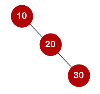
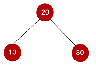
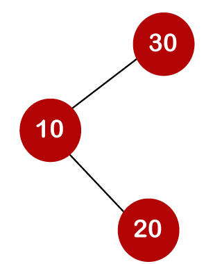
For example, the keys are 10, 20, and 30, and the binary search trees that can be generated from these keys are as follows.
The following is the formula for determining the number of trees:

When we utilize the above calculation, we discover that we can make a total of 5 trees.
The cost of looking for an element is determined by the comparisons that must be done. Now we'll figure out what the average time cost of the above binary search trees is.

A total of three comparisons may be made in the tree above. The average number of comparisons is calculated as follows:

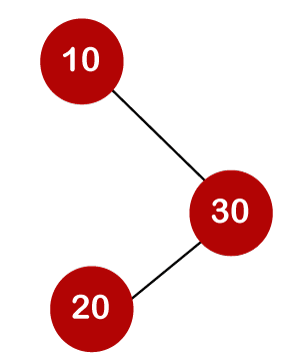
The average number of comparisons that can be made in the above tree is:


The average number of comparisons that can be made in the above tree is:


The total number of comparisons in the tree above is three. As a result, the average number of possible comparisons is:

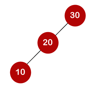
The total number of comparisons in the tree above is three. As a result, the average number of possible comparisons is:

The number of comparisons is lower in the third example since the tree's height is lower, hence it's a balanced binary search tree.
It is a general algorithmic technique
● Backtracking algorithm is used to solve a problem recursively to get a solution incrementally.
● It is used to solve problems when the sequence of objects is chosen from a specified set so that the sequence can satisfy some criteria.
● Backtracking is the systematic method which helps to try out a sequence of decisions until you find out that solution.
● It starts with one smaller piece at a time, if its solution fails to satisfy the constraint then it can be removed at any point of time.
● It searches for any possible combination in order to solve a computational problem.

Fig 2: a - backtracking
However, we usually design our trees from the top down, with the root at the bottom.

Fig 3: Backtracking
Nodes are the building blocks of a tree.

Fig 4: Backtracking
Backtracking is similar to searching a tree for a certain "target" leaf node.
Backtracking is straightforward: we "examine" each node as follows:
To "explore" node N:
1. If N is a goal node, return "success"
2. If N is a leaf node, return "failure"
3. For each child C of N,
Explore C
If C was successful, return "success"
4. Return "failure"
Two constraints:
- Implicit constraint
- Explicit constraint
The backtracking algorithm finds the solution by scanning the solution space for the given problem in a systematic manner. With any bounding function, backtracking is a depth-first search. All backtracking solutions are required to fulfill a complex set of restrictions. Constraints might be stated explicitly or implicitly.
The Explicit Constraint is enforced, which limits each vector element's selection to the supplied set.
Implicit Constraint is ruled, which determines which each of the tuples in the solution space actually satisfy the criterion function.
Application:
- N-queen problem
- Sum of subset
- Graph coloring
- Hamilton problems
Queen problem
Let chess board having N*N cells.
- We need to place N queens in such a way that no queen is attacked by any other queen.
- The queen can attack horizontally, vertically and diagonally. So initially, we are having N*N unattacked cells where we can place the N queens.
Step 1: Place the first queen at a cell (i,j). Hence the unattacked cell is reduced and the number of queens to be placed is N−1.
Step 2: Place the second queen on an unattacked cell that will reduce the no. Of unattacked cells and no. Of queen to be placed become N-2.
The process continues until it satisfies the following condition.
The no. Of unattacked cell become 0
The no of queens to be placed is not 0.
Step 3: As it satisfies the first condition given above then it’s over, we got a final solution.
But if the unattacked cells become 0, then we need to backtrack and remove the last placed queen from its current place and place it in another cell.
This process will be done recursively.
Example:
8-Queen problem
- The eight-queen problem is the problem of placing eight queens on an 8×8 chessboard such that none of them attack one another.
- The eight-queen puzzle has 92 distinct solutions.
- If a solution that differs only by symmetry operation of the board are counted as one puzzle has 12 unique solutions.
Formulation of problem:
- States: any arrangement of 8 queens on board
- Initial state: 0 queens on the board
- Successor function: add a queen on any square
- Goal state: unattacked 8 queens on the board
Steps to be perform:
- Place the first queen in the left upper corner of the table
- Save the attacked position
- Move to the next queen which can only placed on next line
- Search for a valid position. (unattacked position) If there is one go to step 8.
- There is not a valid position for a queen then delete it.
- Move to the previous queen
- Got to step 4
- Place it to the first valid position
- Save the attacked positions
- If the queen processed is the last stop otherwise go to step 3.
Algorithm:
PutQueen(row)
{
For every position col on the same row
If the position col is available
Place the next queen in position col
If(row<8)
putQueen(row+1)
Else success
Remove the queen from positioncol
}
Key takeaway
- Backtracking algorithm is used to solve a problem recursively to get a solution incrementally.
- It is used to solve problems when the sequence of objects is chosen from a specified set so that the sequence can satisfy some criteria.
We must use the Backtracking technique to identify the Hamiltonian Circuit given a graph G = (V, E). We begin our search at any random vertex, such as 'a.' The root of our implicit tree is this vertex 'a.' The first intermediate vertex of the Hamiltonian Cycle to be constructed is the first element of our partial solution. By alphabetical order, the next nearby vertex is chosen.
A dead end is reached when any arbitrary vertices forms a cycle with any vertex other than vertex 'a' at any point. In this situation, we backtrack one step and restart the search by selecting a new vertex and backtracking the partial element; the answer must be removed. If a Hamiltonian Cycle is found, the backtracking search is successful.
Example - Consider the graph G = (V, E) in fig. We must use the Backtracking method to find a Hamiltonian circuit.

To begin, we'll start with vertex 'a,' which will serve as the root of our implicit tree.

Following that, we select the vertex 'b' adjacent to 'a' because it is the first in lexicographical order (b, c, d).

Then, next to 'b,' we select 'c.'

Next, we choose the letter 'd,' which is adjacent to the letter 'c.'

Then we select the letter 'e,' which is adjacent to the letter 'd.'

Then, adjacent to 'e,' we select vertex 'f.' D and e are the vertex next to 'f,' but they've already been there. As a result, we reach a dead end and go back a step to delete the vertex 'f' from the partial solution.
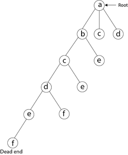
The vertices adjacent to 'e' is b, c, d, and f, from which vertex 'f' has already been verified, and b, c, and d have previously been visited, according to backtracking. As a result, we go back one step. The vertex adjacent to d is now e, f, from which e has already been checked, and the vertex adjacent to 'f' is now d and e. We get a dead state if we revisit the 'e' vertex. As a result, we go back one step.
References:
- Analysis and Design of Algorithms: A Beginner's Approach, by Rajesh K. Shukla, Wiley Publications
- “Algorithms, Data Structuresand Problem Solving with C++”, Illustrated Edition by Mark Allen Weiss, Addison-Wesley Publishing Company.
- Data structures and Algorithm Analysis in C, 2nd edition, M.A.Weiss, Pearson
- Data Structures with C, Seymour Lipschutz, Schaum's Outlines, Tata McGraw Hill Education.
Unit - 5
Algorithms
Advanced data structures are one of the most important areas of data science since they are used to store, organize, and manage data and information in order to make it more efficient, accessible, and modifiable. They serve as the foundation for creating efficient and successful software and algorithms. Being a skilled programmer necessitates knowing how to develop and construct a good data structure. Its scope is also expanding as new information technology and working techniques emerge.
Many algorithms' efficiency and performance are directly proportional to the data they use to perform calculations and other data operations. Data structures perform the basic function of keeping data in main memory during run-time or programme execution, hence memory management is particularly significant since it has a direct impact on the space complexity of a programme or algorithm. As a result, selecting a suitable data structure is critical to programme efficiency and performance.
List of Advanced Data Structures
Advanced-Data structures have multiplied into a plethora of manifolds. The following are the broad categories into which sophisticated data structures are classified:
● Primitive types
● Composite or non-primitive type
● Abstract data types
● Linear Data Structures
● Tree types
● Hash-based structures
● Graphs
It is a greedy algorithm that solves the single-source shortest path problem for a directed graph G = (V, E) with nonnegative edge weights, i.e., w (u, v) ≥ 0 for each edge (u, v) ∈ E.
Dijkstra's Algorithm maintains a set S of vertices whose final shortest - path weights from the source s have already been determined. That's for all vertices v ∈ S; we have d [v] = δ (s, v). The algorithm repeatedly selects the vertex u ∈ V - S with the minimum shortest - path estimate, insert u into S and relaxes all edges leaving u.
Because it always chooses the "lightest" or "closest" vertex in V - S to insert into set S, it is called as the greedy strategy.
Dijkstra's Algorithm (G, w, s)
1. INITIALIZE - SINGLE - SOURCE (G, s)
2. S←∅
3. Q←V [G]
4. While Q ≠ ∅
5. Do u ← EXTRACT - MIN (Q)
6. S ← S ∪ {u}
7. For each vertex v ∈ Adj [u]
8. Do RELAX (u, v, w)
Analysis: The running time of Dijkstra's algorithm on a graph with edges E and vertices V can be expressed as a function of |E| and |V| using the Big - O notation. The simplest implementation of the Dijkstra's algorithm stores vertices of set Q in an ordinary linked list or array, and operation Extract - Min (Q) is simply a linear search through all vertices in Q. In this case, the running time is O (|V2 |+|E|=O(V2 ).
Example:

Solution:
Step1: Q =[s, t, x, y, z]
We scanned vertices one by one and find out its adjacent. Calculate the distance of each adjacent to the source vertices.
We make a stack, which contains those vertices which are selected after computation of shortest distance.
Firstly we take's' in stack M (which is a source)
- M = [S] Q = [t, x, y, z]
Step 2: Now find the adjacent of s that are t and y.
- Adj [s] → t, y [Here s is u and t and y are v]

Case - (i) s → t
d [v] > d [u] + w [u, v]
d [t] > d [s] + w [s, t]
∞ > 0 + 10 [false condition]
Then d [t] ← 10
π [t] ← 5
Adj [s] ← t, y
Case - (ii) s→ y
d [v] > d [u] + w [u, v]
d [y] > d [s] + w [s, y]
∞ > 0 + 5 [false condition]
∞ > 5
Then d [y] ← 5
π [y] ← 5
By comparing case (i) and case (ii)
Adj [s] → t = 10, y = 5
y is shortest
y is assigned in 5 = [s, y]

Step 3: Now find the adjacent of y that is t, x, z.
- Adj [y] → t, x, z [Here y is u and t, x, z are v]
Case - (i) y →t
d [v] > d [u] + w [u, v]
d [t] > d [y] + w [y, t]
10 > 5 + 3
10 > 8
Then d [t] ← 8
π [t] ← y
Case - (ii) y → x
d [v] > d [u] + w [u, v]
d [x] > d [y] + w [y, x]
∞ > 5 + 9
∞ > 14
Then d [x] ← 14
π [x] ← 14
Case - (iii) y → z
d [v] > d [u] + w [u, v]
d [z] > d [y] + w [y, z]
∞ > 5 + 2
∞ > 7
Then d [z] ← 7
π [z] ← y
By comparing case (i), case (ii) and case (iii)
Adj [y] → x = 14, t = 8, z =7
z is shortest
z is assigned in 7 = [s, z]
Step - 4 Now we will find adj [z] that are s, x
- Adj [z] → [x, s] [Here z is u and s and x are v]
Case - (i) z → x
d [v] > d [u] + w [u, v]
d [x] > d [z] + w [z, x]
14 > 7 + 6
14 > 13
Then d [x] ← 13
π [x] ← z
Case - (ii) z → s
d [v] > d [u] + w [u, v]
d [s] > d [z] + w [z, s]
0 > 7 + 7
0 > 14
∴ This condition does not satisfy so it will be discarded.
Now we have x = 13.

Step 5: Now we will find Adj [t]
Adj [t] → [x, y] [Here t is u and x and y are v]
Case - (i) t → x
d [v] > d [u] + w [u, v]
d [x] > d [t] + w [t, x]
13 > 8 + 1
13 > 9
Then d [x] ← 9
π [x] ← t
Case - (ii) t → y
d [v] > d [u] + w [u, v]
d [y] > d [t] + w [t, y]
5 > 10
∴ This condition does not satisfy so it will be discarded.

Thus, we get all shortest path vertex as
Weight from s to y is 5
Weight from s to z is 7
Weight from s to t is 8
Weight from s to x is 9
These are the shortest distance from the source's' in the given graph.

Disadvantage of Dijkstra's Algorithm:
- It does a blind search, so wastes a lot of time while processing.
- It can't handle negative edges.
- It leads to the acyclic graph and most often cannot obtain the right shortest path.
- We need to keep track of vertices that have been visited.
In Dijkstra’s algorithm, two sets are maintained, one set contains list of vertices already included in SPT (Shortest Path Tree), other set contains vertices not yet included. With adjacency list representation, all vertices of a graph can be traversed in O(V+E) time using BFS. The idea is to traverse all vertices of graph using BFS and use a Min Heap to store the vertices not yet included in SPT (or the vertices for which shortest distance is not finalized yet).
Min Heap is used as a priority queue to get the minimum distance vertex from set of not yet included vertices. Time complexity of operations like extract-min and decrease-key value is O(LogV) for Min Heap.
Following are the detailed steps.
1) Create a Min Heap of size V where V is the number of vertices in the given graph. Every node of min heap contains vertex number and distance value of the vertex.
2) Initialize Min Heap with source vertex as root (the distance value assigned to source vertex is 0). The distance value assigned to all other vertices is INF (infinite).
3) While Min Heap is not empty, do following
a) Extract the vertex with minimum distance value node from Min Heap. Let the extracted vertex be u.
b) For every adjacent vertex v of u, check if v is in Min Heap. If v is in Min Heap and distance value is more than weight of u-v plus distance value of u, then update the distance value of v.
Let us understand with the following example. Let the given source vertex be 0

Initially, distance value of source vertex is 0 and INF (infinite) for all other vertices. So source vertex is extracted from Min Heap and distance values of vertices adjacent to 0 (1 and 7) are updated. Min Heap contains all vertices except vertex 0.
The vertices in green color are the vertices for which minimum distances are finalized and are not in Min Heap

Since distance value of vertex 1 is minimum among all nodes in Min Heap, it is extracted from Min Heap and distance values of vertices adjacent to 1 are updated (distance is updated if the vertex is in Min Heap and distance through 1 is shorter than the previous distance). Min Heap contains all vertices except vertex 0 and 1.

Pick the vertex with minimum distance value from min heap. Vertex 7 is picked. So min heap now contains all vertices except 0, 1 and 7. Update the distance values of adjacent vertices of 7. The distance value of vertex 6 and 8 becomes finite (15 and 9 respectively).

Pick the vertex with minimum distance from min heap. Vertex 6 is picked. So min heap now contains all vertices except 0, 1, 7 and 6. Update the distance values of adjacent vertices of 6. The distance value of vertex 5 and 8 are updated.

Above steps are repeated till min heap doesn’t become empty. Finally, we get the following shortest path tree.

Key takeaway
- Warshall’s algorithm constructs transitive closure of a given directed graph.
- In directed graphs there are n vertices.
- A graph with each edge directed is called a directed OR digraph graph.
- Dijkstra’s algorithm is the iterative algorithmic process to provide us with the shortest path from one specific starting node to all other nodes of a graph.
It's a weighted graph in which each edge's total weight is negative. A chain is formed when a graph has a negative edge. If the output is negative after performing the chain, the weight and condition will be eliminated. We can't have the shortest path in it if the weight is smaller than negative and -.
In a nutshell, if the output is -ve, both conditions are ignored.
● - ∞
● Not less than 0
We can't have the shortest Path, either.
Example

Beginning from s
Adj [s] = [a, c, e]
Weight from s to a is 3
Let's say we want to find a path from s→c. As a result, we have two path /weight.
s to c = 5, s→c→d→c=8
But s→c is minimum
So s→c = 5
Let's say we want to find a path from s→e. So we're back to having two options.
s→e = 2, s→e→f→e=-1
As -1 < 0 ∴ Condition gets discarded. If we execute this chain, we will get - ∞. So we can't get the shortest path ∴ e = ∞.

The effects of negative weights and the negative weight cycle on the shortest path weights are shown in this diagram.
Because there is only one path from "s to a" (the path <s, a>), δ (s, a) = w (s, a) = 3.
Furthermore, there is only one path from "s to b", so δ (s, b) = w (s, a) + w (a, b) = 3 + (-4) = - 1.
There are an unlimited number of paths from "s to c": <s, c, d, c>, <s, c, d, c, d, c>, and so on. Because the cycle <c, d, c> has a weight of δ(c, d) = w (c, d) + w (d, c) = 6 + (-3) = 3, the shortest path from s to c is s, c>, which has a weight of δ(s, c) = 5.
Similarly, the shortest path from "s to d" is with weight δ (s, d) = w (s, c) + w (s, d) = 11.
Weight (s, d) = w (s, c) + w (s, d) = 11 is also the shortest path from "s to d."
Similarly, there exist an endless number of pathways from s to e:,, and so on. Since the cycle has weight δ (e, f) = w (e, f) + w (f, e) = 3 + (-6) = -3. So - 3 < 0, However, there is no shortest path from s to e, therefore - 3 0. B8y is in the midst of a negative weight cycle. As a result, the path from s to e has arbitrary big negative weights, and δ (s, e) = - ∞.
In the same way, δ (s, f) = - ∞ Because g can be reached via f, we can also find a path from s to g with any large negative weight, and δ (s, g) = - ∞

Negative weight cycle also affects vertices h, I and g. They are also inaccessible from the source node, resulting in a distance of - ∞ to three nodes from the source (h, i, j).
If there are no cycles in a graph, it is called an acyclic graph, and an acyclic graph is the polar opposite of a cyclic graph.

The graph in the preceding figure is acyclic because it has no cycles. That is, if we start from vertex B and tour the graph, there is no single path that will traverse all of the vertices and terminate at the same vertex, which is vertex B.
The following is the most obvious flow network issue:
Problem1: The maximum flow problem aims to discover a flow with the highest value given a flow network G = (V, E).
Problem 2: The maximum flow problem with numerous sources and sinks is similar to the maximum flow problem with a set of {s1,s2,s3.......sn} sources and a set of {t1,t2,t3.......tn} sinks.
Thankfully, this issue isn't as serious as normal maximum flow. We define a new flow network G' by adding additional sources and sinks to the flow network G.
● A super source s,
● A super sink t,
● For each si, add edge (s, si) with capacity ∞, and
● For each ti,add edge (ti,t) with capacity ∞
Figure depicts a flow network with numerous sources and sinks, as well as an analogous single source and sink flow network.

Residual Networks: The Residual Network is made out of a network edge that can accept extra traffic. Assume we have a G = (V, E) flow network with source s and sink t. Examine a pair of vertices u, v ∈ V, and consider f as a flow in G. The residual capacity of (u, v) is the sum of additional net flow we may push from u to v before exceeding the capacity c (u, v).

The residual capacity cf (u,v) is greater than the capacity c when the net flow f (u, v) is negative (u, v).
For Example: if c (u, v) = 16 and f (u, v) =16 and f (u, v) = -4, then the residual capacity cf (u,v) is 20.
Given a flow network G = (V, E) and a flow f, the residual network of G induced by f is Gf = (V, Ef), where

That is, each residual network edge, or residual edge, can permit a net flow that is strictly positive.
Augmenting Path: An augmenting path p is a simple path from s to t in the residual network Gf given a flow network G = (V, E) and a flow f. The residual network approach allows each augmenting path edge (u, v) to accept some additional positive net flow from u to v without violating the edge's capacity constraint.
Let G = (V, E) be a flow network with flow f. The residual capacity of an augmenting path p is

The maximum amount of flow that may be pushed through the augmenting channel is known as the residual capacity. If an augmenting path exists, each of its edges has a positive capacity. This fact will be used to calculate the maximum flow in a flow network.

It is a Dynamic Programming method in which the previous output is used as the input for the next.
Chain denotes that one matrix's column is always equal to the second matrix's row.
Find the most efficient technique to multiply these matrices together given a sequence of matrices. The issue is not so much with performing the multiplications as it is with deciding which sequence to conduct them in.
Because matrix multiplication is associative, we have a lot of alternatives when multiplying a chain of matrices. In other words, the result will be the same regardless of how we parenthesize the product.
For four matrices A, B, C, and D, for example, we would have:
((AB)C)D = ((A(BC))D) = (AB)(CD) = A((BC)D) = A(B(CD))
The number of simple arithmetic operations required to compute the product, or its efficiency, is affected by the order in which we parenthesize the product. Consider the following examples: A is a 10 × 30 matrix, B is a 30 × 5 matrix, and C is a 5 × 60 matrix. Then,
(AB)C = (10×30×5) + (10×5×60) = 1500 + 3000 = 4500 operations
A(BC) = (30×5×60) + (10×30×60) = 9000 + 18000 = 27000 operations.
Obviously, the first parenthesization necessitates fewer processes.
Given an array p[], which depicts a chain of matrices with the ith matrix Ai of dimension p[i-1] x p[i], find the dimension of the ith matrix Ai. MatrixChainOrder() is a function that should return the minimum number of multiplications required to multiply the chain.
Input: p[] = {40, 20, 30, 10, 30}
Output: 26000
40x20, 20x30, 30x10, and 10x30 are the dimensions of the four matrices.
A, B, C, and D are the four input matrices. By using parenthesis in the following method, you can get the smallest amount of multiplications:
(A(BC))D --> 20*30*10 + 40*20*10 + 40*10*30
Input: p[] = {10, 20, 30, 40, 30}
Output: 30000
There are four matrices of 10x20, 20x30, 30x40, and 40x30 dimensions.
A, B, C, and D are the four input matrices. By using parenthesis in the following method, you can get the smallest amount of multiplications:
((AB)C)D --> 10*20*30 + 10*30*40 + 10*40*30
Input: p[] = {10, 20, 30}
Output: 6000
There are just two matrices of 10x20 and 20x30 dimensions. As a result, there is only one way to multiply the matrices, which will cost you 10*20*30.

Fig 1: Example of matrix chain multiplication
Solution for Dynamic Programming:
● Take the matrices sequence and divide it into two subsequences.
● Calculate the cheapest way to multiply each subsequence.
● Add all these expenses, as well as the cost of multiplying the two result matrices.
● Do this for each conceivable split position in the series of matrices, and take the lowest of all of them.
The longest here denotes that the subsequence should be the most significant. The term "common" refers to the fact that some of the characters in the two strings are the same. The term "subsequence" refers to the extraction of some characters from a string that is written in ascending order to generate a subsequence.
Let's look at an example to better grasp the subsequence.
Let's say we have the string 'w'.
W1 = abcd
The subsequences that can be made from the aforementioned string are as follows:
Ab
Bd
Ac
Ad
Acd
Bcd
As all the letters in a sub-string are written in increasing order with respect to their place, the above are the subsequences. If we write ca or da, the subsequence will be incorrect since the characters will not appear in increasing order. The total number of possible subsequences is 2n, where n is the number of characters in a string. Because the value of 'n' in the given string is 4, the total number of subsequences is 16.
W2= bcd
We may deduce that bcd is the longest common subsequence by looking at both strings w1 and w2. If the strings are long, finding the subsequence of each and comparing them to discover the longest common subsequence will be impossible.
LCS Problem Statement:
Determine the length of the longest subsequence in each of two sequences. A subsequence is a series of events that occur in the same order but are not necessarily contiguous. Subsequences of "abcdefg" include "abc", "abg", "bdf", "aeg", "acefg", and so on.
To determine the complexity of the brute force method, we must first determine the number of different subsequences of a string of length n, i.e., the number of subsequences with lengths ranging from 1,2,...n-1. Remember from permutation and combination theory that the number of combinations with one element is nC1. nC2 is the number of combinations with two elements, and so on.
nC0 + nC1 + nC2 +... nCn = 2n, as we know. Because we don't examine the subsequence of length 0, a string of length n has 2n-1 different possible subsequences. As a result, the brute force approach's temporal complexity will be O(n * 2n). It's worth noting that determining if a subsequence is shared by both strings requires O(n) time. Dynamic programming can help with this time complexity.
It's a classic computer science problem that's at the heart of diff (a file comparison programme that shows the differences between two files) and has bioinformatics applications.
Examples:
LCS for input Sequences “ABCDGH” and “AEDFHR” is “ADH” of length 3.
LCS for input Sequences “AGGTAB” and “GXTXAYB” is “GTAB” of length 4.
As we know, the nodes in the left subtree have a lower value than the root node, while the nodes in the right subtree have a higher value than the root node in a binary search tree.
We know the key values of each node in the tree, as well as the frequencies of each node in terms of searching, which is the amount of time it takes to find a node. The overall cost of searching a node is determined by the frequency and key-value. In a variety of applications, the cost of searching is a critical element. The cost of searching a node should be lower overall. Because a balanced binary search tree has fewer levels than the BST, the time required to search a node in the BST is longer. The term "optimal binary search tree" refers to a method of lowering the cost of a binary search tree.
Example
If the keys are 10, 20, 30, 40, 50, 60, 70

All of the nodes on the left subtree are smaller than the root node's value, whereas all of the nodes on the right subtree are greater than the root node's value. The greatest time required to search a node is equal to logn times the tree's minimum height.
Now we'll check how many binary search trees we can make with the quantity of keys we have.
For example, the keys are 10, 20, and 30, and the binary search trees that can be generated from these keys are as follows.
The following is the formula for determining the number of trees:

When we utilize the above calculation, we discover that we can make a total of 5 trees.
The cost of looking for an element is determined by the comparisons that must be done. Now we'll figure out what the average time cost of the above binary search trees is.
A total of three comparisons may be made in the tree above. The average number of comparisons is calculated as follows:


The average number of comparisons that can be made in the above tree is:

The average number of comparisons that can be made in the above tree is:

The total number of comparisons in the tree above is three. As a result, the average number of possible comparisons is:


The total number of comparisons in the tree above is three. As a result, the average number of possible comparisons is:

The number of comparisons is lower in the third example since the tree's height is lower, hence it's a balanced binary search tree.
It is a general algorithmic technique
● Backtracking algorithm is used to solve a problem recursively to get a solution incrementally.
● It is used to solve problems when the sequence of objects is chosen from a specified set so that the sequence can satisfy some criteria.
● Backtracking is the systematic method which helps to try out a sequence of decisions until you find out that solution.
● It starts with one smaller piece at a time, if its solution fails to satisfy the constraint then it can be removed at any point of time.
● It searches for any possible combination in order to solve a computational problem.
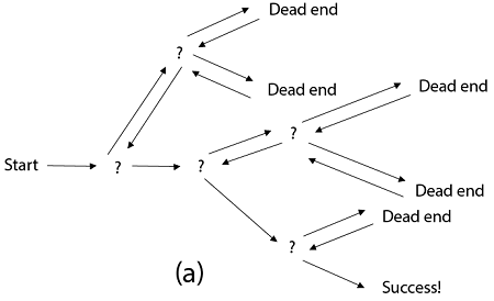
Fig 2: a - backtracking
However, we usually design our trees from the top down, with the root at the bottom.

Fig 3: Backtracking
Nodes are the building blocks of a tree.
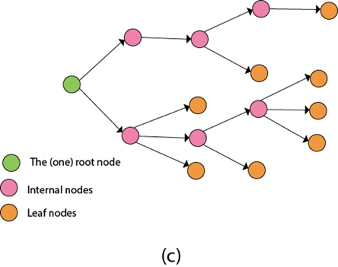
Fig 4: Backtracking
Backtracking is similar to searching a tree for a certain "target" leaf node.
Backtracking is straightforward: we "examine" each node as follows:
To "explore" node N:
1. If N is a goal node, return "success"
2. If N is a leaf node, return "failure"
3. For each child C of N,
Explore C
If C was successful, return "success"
4. Return "failure"
Two constraints:
- Implicit constraint
- Explicit constraint
The backtracking algorithm finds the solution by scanning the solution space for the given problem in a systematic manner. With any bounding function, backtracking is a depth-first search. All backtracking solutions are required to fulfill a complex set of restrictions. Constraints might be stated explicitly or implicitly.
The Explicit Constraint is enforced, which limits each vector element's selection to the supplied set.
Implicit Constraint is ruled, which determines which each of the tuples in the solution space actually satisfy the criterion function.
Application:
- N-queen problem
- Sum of subset
- Graph coloring
- Hamilton problems
Queen problem
Let chess board having N*N cells.
- We need to place N queens in such a way that no queen is attacked by any other queen.
- The queen can attack horizontally, vertically and diagonally. So initially, we are having N*N unattacked cells where we can place the N queens.
Step 1: Place the first queen at a cell (i,j). Hence the unattacked cell is reduced and the number of queens to be placed is N−1.
Step 2: Place the second queen on an unattacked cell that will reduce the no. Of unattacked cells and no. Of queen to be placed become N-2.
The process continues until it satisfies the following condition.
The no. Of unattacked cell become 0
The no of queens to be placed is not 0.
Step 3: As it satisfies the first condition given above then it’s over, we got a final solution.
But if the unattacked cells become 0, then we need to backtrack and remove the last placed queen from its current place and place it in another cell.
This process will be done recursively.
Example:
8-Queen problem
- The eight-queen problem is the problem of placing eight queens on an 8×8 chessboard such that none of them attack one another.
- The eight-queen puzzle has 92 distinct solutions.
- If a solution that differs only by symmetry operation of the board are counted as one puzzle has 12 unique solutions.
Formulation of problem:
- States: any arrangement of 8 queens on board
- Initial state: 0 queens on the board
- Successor function: add a queen on any square
- Goal state: unattacked 8 queens on the board
Steps to be perform:
- Place the first queen in the left upper corner of the table
- Save the attacked position
- Move to the next queen which can only placed on next line
- Search for a valid position. (unattacked position) If there is one go to step 8.
- There is not a valid position for a queen then delete it.
- Move to the previous queen
- Got to step 4
- Place it to the first valid position
- Save the attacked positions
- If the queen processed is the last stop otherwise go to step 3.
Algorithm:
PutQueen(row)
{
For every position col on the same row
If the position col is available
Place the next queen in position col
If(row<8)
putQueen(row+1)
Else success
Remove the queen from positioncol
}
Key takeaway
- Backtracking algorithm is used to solve a problem recursively to get a solution incrementally.
- It is used to solve problems when the sequence of objects is chosen from a specified set so that the sequence can satisfy some criteria.
We must use the Backtracking technique to identify the Hamiltonian Circuit given a graph G = (V, E). We begin our search at any random vertex, such as 'a.' The root of our implicit tree is this vertex 'a.' The first intermediate vertex of the Hamiltonian Cycle to be constructed is the first element of our partial solution. By alphabetical order, the next nearby vertex is chosen.
A dead end is reached when any arbitrary vertices forms a cycle with any vertex other than vertex 'a' at any point. In this situation, we backtrack one step and restart the search by selecting a new vertex and backtracking the partial element; the answer must be removed. If a Hamiltonian Cycle is found, the backtracking search is successful.
Example - Consider the graph G = (V, E) in fig. We must use the Backtracking method to find a Hamiltonian circuit.

To begin, we'll start with vertex 'a,' which will serve as the root of our implicit tree.

Following that, we select the vertex 'b' adjacent to 'a' because it is the first in lexicographical order (b, c, d).

Then, next to 'b,' we select 'c.'

Next, we choose the letter 'd,' which is adjacent to the letter 'c.'

Then we select the letter 'e,' which is adjacent to the letter 'd.'

Then, adjacent to 'e,' we select vertex 'f.' D and e are the vertex next to 'f,' but they've already been there. As a result, we reach a dead end and go back a step to delete the vertex 'f' from the partial solution.

The vertices adjacent to 'e' is b, c, d, and f, from which vertex 'f' has already been verified, and b, c, and d have previously been visited, according to backtracking. As a result, we go back one step. The vertex adjacent to d is now e, f, from which e has already been checked, and the vertex adjacent to 'f' is now d and e. We get a dead state if we revisit the 'e' vertex. As a result, we go back one step.
References:
- Analysis and Design of Algorithms: A Beginner's Approach, by Rajesh K. Shukla, Wiley Publications
- “Algorithms, Data Structuresand Problem Solving with C++”, Illustrated Edition by Mark Allen Weiss, Addison-Wesley Publishing Company.
- Data structures and Algorithm Analysis in C, 2nd edition, M.A.Weiss, Pearson
- Data Structures with C, Seymour Lipschutz, Schaum's Outlines, Tata McGraw Hill Education.
Unit - 5
Algorithms
Advanced data structures are one of the most important areas of data science since they are used to store, organize, and manage data and information in order to make it more efficient, accessible, and modifiable. They serve as the foundation for creating efficient and successful software and algorithms. Being a skilled programmer necessitates knowing how to develop and construct a good data structure. Its scope is also expanding as new information technology and working techniques emerge.
Many algorithms' efficiency and performance are directly proportional to the data they use to perform calculations and other data operations. Data structures perform the basic function of keeping data in main memory during run-time or programme execution, hence memory management is particularly significant since it has a direct impact on the space complexity of a programme or algorithm. As a result, selecting a suitable data structure is critical to programme efficiency and performance.
List of Advanced Data Structures
Advanced-Data structures have multiplied into a plethora of manifolds. The following are the broad categories into which sophisticated data structures are classified:
● Primitive types
● Composite or non-primitive type
● Abstract data types
● Linear Data Structures
● Tree types
● Hash-based structures
● Graphs
It is a greedy algorithm that solves the single-source shortest path problem for a directed graph G = (V, E) with nonnegative edge weights, i.e., w (u, v) ≥ 0 for each edge (u, v) ∈ E.
Dijkstra's Algorithm maintains a set S of vertices whose final shortest - path weights from the source s have already been determined. That's for all vertices v ∈ S; we have d [v] = δ (s, v). The algorithm repeatedly selects the vertex u ∈ V - S with the minimum shortest - path estimate, insert u into S and relaxes all edges leaving u.
Because it always chooses the "lightest" or "closest" vertex in V - S to insert into set S, it is called as the greedy strategy.
Dijkstra's Algorithm (G, w, s)
1. INITIALIZE - SINGLE - SOURCE (G, s)
2. S←∅
3. Q←V [G]
4. While Q ≠ ∅
5. Do u ← EXTRACT - MIN (Q)
6. S ← S ∪ {u}
7. For each vertex v ∈ Adj [u]
8. Do RELAX (u, v, w)
Analysis: The running time of Dijkstra's algorithm on a graph with edges E and vertices V can be expressed as a function of |E| and |V| using the Big - O notation. The simplest implementation of the Dijkstra's algorithm stores vertices of set Q in an ordinary linked list or array, and operation Extract - Min (Q) is simply a linear search through all vertices in Q. In this case, the running time is O (|V2 |+|E|=O(V2 ).
Example:

Solution:
Step1: Q =[s, t, x, y, z]
We scanned vertices one by one and find out its adjacent. Calculate the distance of each adjacent to the source vertices.
We make a stack, which contains those vertices which are selected after computation of shortest distance.
Firstly we take's' in stack M (which is a source)
- M = [S] Q = [t, x, y, z]
Step 2: Now find the adjacent of s that are t and y.
- Adj [s] → t, y [Here s is u and t and y are v]

Case - (i) s → t
d [v] > d [u] + w [u, v]
d [t] > d [s] + w [s, t]
∞ > 0 + 10 [false condition]
Then d [t] ← 10
π [t] ← 5
Adj [s] ← t, y
Case - (ii) s→ y
d [v] > d [u] + w [u, v]
d [y] > d [s] + w [s, y]
∞ > 0 + 5 [false condition]
∞ > 5
Then d [y] ← 5
π [y] ← 5
By comparing case (i) and case (ii)
Adj [s] → t = 10, y = 5
y is shortest
y is assigned in 5 = [s, y]

Step 3: Now find the adjacent of y that is t, x, z.
- Adj [y] → t, x, z [Here y is u and t, x, z are v]
Case - (i) y →t
d [v] > d [u] + w [u, v]
d [t] > d [y] + w [y, t]
10 > 5 + 3
10 > 8
Then d [t] ← 8
π [t] ← y
Case - (ii) y → x
d [v] > d [u] + w [u, v]
d [x] > d [y] + w [y, x]
∞ > 5 + 9
∞ > 14
Then d [x] ← 14
π [x] ← 14
Case - (iii) y → z
d [v] > d [u] + w [u, v]
d [z] > d [y] + w [y, z]
∞ > 5 + 2
∞ > 7
Then d [z] ← 7
π [z] ← y
By comparing case (i), case (ii) and case (iii)
Adj [y] → x = 14, t = 8, z =7
z is shortest
z is assigned in 7 = [s, z]

Step - 4 Now we will find adj [z] that are s, x
- Adj [z] → [x, s] [Here z is u and s and x are v]
Case - (i) z → x
d [v] > d [u] + w [u, v]
d [x] > d [z] + w [z, x]
14 > 7 + 6
14 > 13
Then d [x] ← 13
π [x] ← z
Case - (ii) z → s
d [v] > d [u] + w [u, v]
d [s] > d [z] + w [z, s]
0 > 7 + 7
0 > 14
∴ This condition does not satisfy so it will be discarded.
Now we have x = 13.
Step 5: Now we will find Adj [t]
Adj [t] → [x, y] [Here t is u and x and y are v]
Case - (i) t → x
d [v] > d [u] + w [u, v]
d [x] > d [t] + w [t, x]
13 > 8 + 1
13 > 9
Then d [x] ← 9
π [x] ← t
Case - (ii) t → y
d [v] > d [u] + w [u, v]
d [y] > d [t] + w [t, y]
5 > 10
∴ This condition does not satisfy so it will be discarded.
Thus, we get all shortest path vertex as
Weight from s to y is 5
Weight from s to z is 7
Weight from s to t is 8
Weight from s to x is 9
These are the shortest distance from the source's' in the given graph.
Disadvantage of Dijkstra's Algorithm:
- It does a blind search, so wastes a lot of time while processing.
- It can't handle negative edges.
- It leads to the acyclic graph and most often cannot obtain the right shortest path.
- We need to keep track of vertices that have been visited.
In Dijkstra’s algorithm, two sets are maintained, one set contains list of vertices already included in SPT (Shortest Path Tree), other set contains vertices not yet included. With adjacency list representation, all vertices of a graph can be traversed in O(V+E) time using BFS. The idea is to traverse all vertices of graph using BFS and use a Min Heap to store the vertices not yet included in SPT (or the vertices for which shortest distance is not finalized yet).
Min Heap is used as a priority queue to get the minimum distance vertex from set of not yet included vertices. Time complexity of operations like extract-min and decrease-key value is O(LogV) for Min Heap.
Following are the detailed steps.
1) Create a Min Heap of size V where V is the number of vertices in the given graph. Every node of min heap contains vertex number and distance value of the vertex.
2) Initialize Min Heap with source vertex as root (the distance value assigned to source vertex is 0). The distance value assigned to all other vertices is INF (infinite).
3) While Min Heap is not empty, do following
a) Extract the vertex with minimum distance value node from Min Heap. Let the extracted vertex be u.
b) For every adjacent vertex v of u, check if v is in Min Heap. If v is in Min Heap and distance value is more than weight of u-v plus distance value of u, then update the distance value of v.
Let us understand with the following example. Let the given source vertex be 0

Initially, distance value of source vertex is 0 and INF (infinite) for all other vertices. So source vertex is extracted from Min Heap and distance values of vertices adjacent to 0 (1 and 7) are updated. Min Heap contains all vertices except vertex 0.
The vertices in green color are the vertices for which minimum distances are finalized and are not in Min Heap

Since distance value of vertex 1 is minimum among all nodes in Min Heap, it is extracted from Min Heap and distance values of vertices adjacent to 1 are updated (distance is updated if the vertex is in Min Heap and distance through 1 is shorter than the previous distance). Min Heap contains all vertices except vertex 0 and 1.

Pick the vertex with minimum distance value from min heap. Vertex 7 is picked. So min heap now contains all vertices except 0, 1 and 7. Update the distance values of adjacent vertices of 7. The distance value of vertex 6 and 8 becomes finite (15 and 9 respectively).

Pick the vertex with minimum distance from min heap. Vertex 6 is picked. So min heap now contains all vertices except 0, 1, 7 and 6. Update the distance values of adjacent vertices of 6. The distance value of vertex 5 and 8 are updated.

Above steps are repeated till min heap doesn’t become empty. Finally, we get the following shortest path tree.

Key takeaway
- Warshall’s algorithm constructs transitive closure of a given directed graph.
- In directed graphs there are n vertices.
- A graph with each edge directed is called a directed OR digraph graph.
- Dijkstra’s algorithm is the iterative algorithmic process to provide us with the shortest path from one specific starting node to all other nodes of a graph.
It's a weighted graph in which each edge's total weight is negative. A chain is formed when a graph has a negative edge. If the output is negative after performing the chain, the weight and condition will be eliminated. We can't have the shortest path in it if the weight is smaller than negative and -.
In a nutshell, if the output is -ve, both conditions are ignored.
● - ∞
● Not less than 0
We can't have the shortest Path, either.
Example

Beginning from s
Adj [s] = [a, c, e]
Weight from s to a is 3
Let's say we want to find a path from s→c. As a result, we have two path /weight.
s to c = 5, s→c→d→c=8
But s→c is minimum
So s→c = 5
Let's say we want to find a path from s→e. So we're back to having two options.
s→e = 2, s→e→f→e=-1
As -1 < 0 ∴ Condition gets discarded. If we execute this chain, we will get - ∞. So we can't get the shortest path ∴ e = ∞.

The effects of negative weights and the negative weight cycle on the shortest path weights are shown in this diagram.
Because there is only one path from "s to a" (the path <s, a>), δ (s, a) = w (s, a) = 3.
Furthermore, there is only one path from "s to b", so δ (s, b) = w (s, a) + w (a, b) = 3 + (-4) = - 1.
There are an unlimited number of paths from "s to c": <s, c, d, c>, <s, c, d, c, d, c>, and so on. Because the cycle <c, d, c> has a weight of δ(c, d) = w (c, d) + w (d, c) = 6 + (-3) = 3, the shortest path from s to c is s, c>, which has a weight of δ(s, c) = 5.
Similarly, the shortest path from "s to d" is with weight δ (s, d) = w (s, c) + w (s, d) = 11.
Weight (s, d) = w (s, c) + w (s, d) = 11 is also the shortest path from "s to d."
Similarly, there exist an endless number of pathways from s to e:,, and so on. Since the cycle has weight δ (e, f) = w (e, f) + w (f, e) = 3 + (-6) = -3. So - 3 < 0, However, there is no shortest path from s to e, therefore - 3 0. B8y is in the midst of a negative weight cycle. As a result, the path from s to e has arbitrary big negative weights, and δ (s, e) = - ∞.
In the same way, δ (s, f) = - ∞ Because g can be reached via f, we can also find a path from s to g with any large negative weight, and δ (s, g) = - ∞
Negative weight cycle also affects vertices h, I and g. They are also inaccessible from the source node, resulting in a distance of - ∞ to three nodes from the source (h, i, j).
If there are no cycles in a graph, it is called an acyclic graph, and an acyclic graph is the polar opposite of a cyclic graph.

The graph in the preceding figure is acyclic because it has no cycles. That is, if we start from vertex B and tour the graph, there is no single path that will traverse all of the vertices and terminate at the same vertex, which is vertex B.
The following is the most obvious flow network issue:
Problem1: The maximum flow problem aims to discover a flow with the highest value given a flow network G = (V, E).
Problem 2: The maximum flow problem with numerous sources and sinks is similar to the maximum flow problem with a set of {s1,s2,s3.......sn} sources and a set of {t1,t2,t3.......tn} sinks.
Thankfully, this issue isn't as serious as normal maximum flow. We define a new flow network G' by adding additional sources and sinks to the flow network G.
● A super source s,
● A super sink t,
● For each si, add edge (s, si) with capacity ∞, and
● For each ti,add edge (ti,t) with capacity ∞
Figure depicts a flow network with numerous sources and sinks, as well as an analogous single source and sink flow network.
Residual Networks: The Residual Network is made out of a network edge that can accept extra traffic. Assume we have a G = (V, E) flow network with source s and sink t. Examine a pair of vertices u, v ∈ V, and consider f as a flow in G. The residual capacity of (u, v) is the sum of additional net flow we may push from u to v before exceeding the capacity c (u, v).

The residual capacity cf (u,v) is greater than the capacity c when the net flow f (u, v) is negative (u, v).
For Example: if c (u, v) = 16 and f (u, v) =16 and f (u, v) = -4, then the residual capacity cf (u,v) is 20.
Given a flow network G = (V, E) and a flow f, the residual network of G induced by f is Gf = (V, Ef), where

That is, each residual network edge, or residual edge, can permit a net flow that is strictly positive.
Augmenting Path: An augmenting path p is a simple path from s to t in the residual network Gf given a flow network G = (V, E) and a flow f. The residual network approach allows each augmenting path edge (u, v) to accept some additional positive net flow from u to v without violating the edge's capacity constraint.
Let G = (V, E) be a flow network with flow f. The residual capacity of an augmenting path p is

The maximum amount of flow that may be pushed through the augmenting channel is known as the residual capacity. If an augmenting path exists, each of its edges has a positive capacity. This fact will be used to calculate the maximum flow in a flow network.

It is a Dynamic Programming method in which the previous output is used as the input for the next.
Chain denotes that one matrix's column is always equal to the second matrix's row.
Find the most efficient technique to multiply these matrices together given a sequence of matrices. The issue is not so much with performing the multiplications as it is with deciding which sequence to conduct them in.
Because matrix multiplication is associative, we have a lot of alternatives when multiplying a chain of matrices. In other words, the result will be the same regardless of how we parenthesize the product.
For four matrices A, B, C, and D, for example, we would have:
((AB)C)D = ((A(BC))D) = (AB)(CD) = A((BC)D) = A(B(CD))
The number of simple arithmetic operations required to compute the product, or its efficiency, is affected by the order in which we parenthesize the product. Consider the following examples: A is a 10 × 30 matrix, B is a 30 × 5 matrix, and C is a 5 × 60 matrix. Then,
(AB)C = (10×30×5) + (10×5×60) = 1500 + 3000 = 4500 operations
A(BC) = (30×5×60) + (10×30×60) = 9000 + 18000 = 27000 operations.
Obviously, the first parenthesization necessitates fewer processes.
Given an array p[], which depicts a chain of matrices with the ith matrix Ai of dimension p[i-1] x p[i], find the dimension of the ith matrix Ai. MatrixChainOrder() is a function that should return the minimum number of multiplications required to multiply the chain.
Input: p[] = {40, 20, 30, 10, 30}
Output: 26000
40x20, 20x30, 30x10, and 10x30 are the dimensions of the four matrices.
A, B, C, and D are the four input matrices. By using parenthesis in the following method, you can get the smallest amount of multiplications:
(A(BC))D --> 20*30*10 + 40*20*10 + 40*10*30
Input: p[] = {10, 20, 30, 40, 30}
Output: 30000
There are four matrices of 10x20, 20x30, 30x40, and 40x30 dimensions.
A, B, C, and D are the four input matrices. By using parenthesis in the following method, you can get the smallest amount of multiplications:
((AB)C)D --> 10*20*30 + 10*30*40 + 10*40*30
Input: p[] = {10, 20, 30}
Output: 6000
There are just two matrices of 10x20 and 20x30 dimensions. As a result, there is only one way to multiply the matrices, which will cost you 10*20*30.

Fig 1: Example of matrix chain multiplication
Solution for Dynamic Programming:
● Take the matrices sequence and divide it into two subsequences.
● Calculate the cheapest way to multiply each subsequence.
● Add all these expenses, as well as the cost of multiplying the two result matrices.
● Do this for each conceivable split position in the series of matrices, and take the lowest of all of them.
The longest here denotes that the subsequence should be the most significant. The term "common" refers to the fact that some of the characters in the two strings are the same. The term "subsequence" refers to the extraction of some characters from a string that is written in ascending order to generate a subsequence.
Let's look at an example to better grasp the subsequence.
Let's say we have the string 'w'.
W1 = abcd
The subsequences that can be made from the aforementioned string are as follows:
Ab
Bd
Ac
Ad
Acd
Bcd
As all the letters in a sub-string are written in increasing order with respect to their place, the above are the subsequences. If we write ca or da, the subsequence will be incorrect since the characters will not appear in increasing order. The total number of possible subsequences is 2n, where n is the number of characters in a string. Because the value of 'n' in the given string is 4, the total number of subsequences is 16.
W2= bcd
We may deduce that bcd is the longest common subsequence by looking at both strings w1 and w2. If the strings are long, finding the subsequence of each and comparing them to discover the longest common subsequence will be impossible.
LCS Problem Statement:
Determine the length of the longest subsequence in each of two sequences. A subsequence is a series of events that occur in the same order but are not necessarily contiguous. Subsequences of "abcdefg" include "abc", "abg", "bdf", "aeg", "acefg", and so on.
To determine the complexity of the brute force method, we must first determine the number of different subsequences of a string of length n, i.e., the number of subsequences with lengths ranging from 1,2,...n-1. Remember from permutation and combination theory that the number of combinations with one element is nC1. nC2 is the number of combinations with two elements, and so on.
nC0 + nC1 + nC2 +... nCn = 2n, as we know. Because we don't examine the subsequence of length 0, a string of length n has 2n-1 different possible subsequences. As a result, the brute force approach's temporal complexity will be O(n * 2n). It's worth noting that determining if a subsequence is shared by both strings requires O(n) time. Dynamic programming can help with this time complexity.
It's a classic computer science problem that's at the heart of diff (a file comparison programme that shows the differences between two files) and has bioinformatics applications.
Examples:
LCS for input Sequences “ABCDGH” and “AEDFHR” is “ADH” of length 3.
LCS for input Sequences “AGGTAB” and “GXTXAYB” is “GTAB” of length 4.
As we know, the nodes in the left subtree have a lower value than the root node, while the nodes in the right subtree have a higher value than the root node in a binary search tree.
We know the key values of each node in the tree, as well as the frequencies of each node in terms of searching, which is the amount of time it takes to find a node. The overall cost of searching a node is determined by the frequency and key-value. In a variety of applications, the cost of searching is a critical element. The cost of searching a node should be lower overall. Because a balanced binary search tree has fewer levels than the BST, the time required to search a node in the BST is longer. The term "optimal binary search tree" refers to a method of lowering the cost of a binary search tree.
Example
If the keys are 10, 20, 30, 40, 50, 60, 70
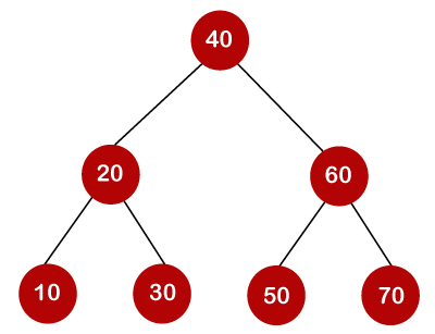
All of the nodes on the left subtree are smaller than the root node's value, whereas all of the nodes on the right subtree are greater than the root node's value. The greatest time required to search a node is equal to logn times the tree's minimum height.
Now we'll check how many binary search trees we can make with the quantity of keys we have.
For example, the keys are 10, 20, and 30, and the binary search trees that can be generated from these keys are as follows.
The following is the formula for determining the number of trees:
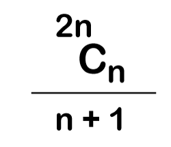
When we utilize the above calculation, we discover that we can make a total of 5 trees.
The cost of looking for an element is determined by the comparisons that must be done. Now we'll figure out what the average time cost of the above binary search trees is.

A total of three comparisons may be made in the tree above. The average number of comparisons is calculated as follows:


The average number of comparisons that can be made in the above tree is:


The average number of comparisons that can be made in the above tree is:


The total number of comparisons in the tree above is three. As a result, the average number of possible comparisons is:


The total number of comparisons in the tree above is three. As a result, the average number of possible comparisons is:

The number of comparisons is lower in the third example since the tree's height is lower, hence it's a balanced binary search tree.
It is a general algorithmic technique
● Backtracking algorithm is used to solve a problem recursively to get a solution incrementally.
● It is used to solve problems when the sequence of objects is chosen from a specified set so that the sequence can satisfy some criteria.
● Backtracking is the systematic method which helps to try out a sequence of decisions until you find out that solution.
● It starts with one smaller piece at a time, if its solution fails to satisfy the constraint then it can be removed at any point of time.
● It searches for any possible combination in order to solve a computational problem.

Fig 2: a - backtracking
However, we usually design our trees from the top down, with the root at the bottom.
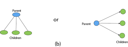
Fig 3: Backtracking
Nodes are the building blocks of a tree.

Fig 4: Backtracking
Backtracking is similar to searching a tree for a certain "target" leaf node.
Backtracking is straightforward: we "examine" each node as follows:
To "explore" node N:
1. If N is a goal node, return "success"
2. If N is a leaf node, return "failure"
3. For each child C of N,
Explore C
If C was successful, return "success"
4. Return "failure"
Two constraints:
- Implicit constraint
- Explicit constraint
The backtracking algorithm finds the solution by scanning the solution space for the given problem in a systematic manner. With any bounding function, backtracking is a depth-first search. All backtracking solutions are required to fulfill a complex set of restrictions. Constraints might be stated explicitly or implicitly.
The Explicit Constraint is enforced, which limits each vector element's selection to the supplied set.
Implicit Constraint is ruled, which determines which each of the tuples in the solution space actually satisfy the criterion function.
Application:
- N-queen problem
- Sum of subset
- Graph coloring
- Hamilton problems
Queen problem
Let chess board having N*N cells.
- We need to place N queens in such a way that no queen is attacked by any other queen.
- The queen can attack horizontally, vertically and diagonally. So initially, we are having N*N unattacked cells where we can place the N queens.
Step 1: Place the first queen at a cell (i,j). Hence the unattacked cell is reduced and the number of queens to be placed is N−1.
Step 2: Place the second queen on an unattacked cell that will reduce the no. Of unattacked cells and no. Of queen to be placed become N-2.
The process continues until it satisfies the following condition.
The no. Of unattacked cell become 0
The no of queens to be placed is not 0.
Step 3: As it satisfies the first condition given above then it’s over, we got a final solution.
But if the unattacked cells become 0, then we need to backtrack and remove the last placed queen from its current place and place it in another cell.
This process will be done recursively.
Example:
8-Queen problem
- The eight-queen problem is the problem of placing eight queens on an 8×8 chessboard such that none of them attack one another.
- The eight-queen puzzle has 92 distinct solutions.
- If a solution that differs only by symmetry operation of the board are counted as one puzzle has 12 unique solutions.
Formulation of problem:
- States: any arrangement of 8 queens on board
- Initial state: 0 queens on the board
- Successor function: add a queen on any square
- Goal state: unattacked 8 queens on the board
Steps to be perform:
- Place the first queen in the left upper corner of the table
- Save the attacked position
- Move to the next queen which can only placed on next line
- Search for a valid position. (unattacked position) If there is one go to step 8.
- There is not a valid position for a queen then delete it.
- Move to the previous queen
- Got to step 4
- Place it to the first valid position
- Save the attacked positions
- If the queen processed is the last stop otherwise go to step 3.
Algorithm:
PutQueen(row)
{
For every position col on the same row
If the position col is available
Place the next queen in position col
If(row<8)
putQueen(row+1)
Else success
Remove the queen from positioncol
}
Key takeaway
- Backtracking algorithm is used to solve a problem recursively to get a solution incrementally.
- It is used to solve problems when the sequence of objects is chosen from a specified set so that the sequence can satisfy some criteria.
We must use the Backtracking technique to identify the Hamiltonian Circuit given a graph G = (V, E). We begin our search at any random vertex, such as 'a.' The root of our implicit tree is this vertex 'a.' The first intermediate vertex of the Hamiltonian Cycle to be constructed is the first element of our partial solution. By alphabetical order, the next nearby vertex is chosen.
A dead end is reached when any arbitrary vertices forms a cycle with any vertex other than vertex 'a' at any point. In this situation, we backtrack one step and restart the search by selecting a new vertex and backtracking the partial element; the answer must be removed. If a Hamiltonian Cycle is found, the backtracking search is successful.
Example - Consider the graph G = (V, E) in fig. We must use the Backtracking method to find a Hamiltonian circuit.
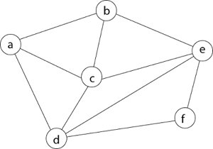
To begin, we'll start with vertex 'a,' which will serve as the root of our implicit tree.

Following that, we select the vertex 'b' adjacent to 'a' because it is the first in lexicographical order (b, c, d).

Then, next to 'b,' we select 'c.'

Next, we choose the letter 'd,' which is adjacent to the letter 'c.'

Then we select the letter 'e,' which is adjacent to the letter 'd.'

Then, adjacent to 'e,' we select vertex 'f.' D and e are the vertex next to 'f,' but they've already been there. As a result, we reach a dead end and go back a step to delete the vertex 'f' from the partial solution.

The vertices adjacent to 'e' is b, c, d, and f, from which vertex 'f' has already been verified, and b, c, and d have previously been visited, according to backtracking. As a result, we go back one step. The vertex adjacent to d is now e, f, from which e has already been checked, and the vertex adjacent to 'f' is now d and e. We get a dead state if we revisit the 'e' vertex. As a result, we go back one step.
References:
- Analysis and Design of Algorithms: A Beginner's Approach, by Rajesh K. Shukla, Wiley Publications
- “Algorithms, Data Structuresand Problem Solving with C++”, Illustrated Edition by Mark Allen Weiss, Addison-Wesley Publishing Company.
- Data structures and Algorithm Analysis in C, 2nd edition, M.A.Weiss, Pearson
- Data Structures with C, Seymour Lipschutz, Schaum's Outlines, Tata McGraw Hill Education.
Unit - 5
Algorithms
Advanced data structures are one of the most important areas of data science since they are used to store, organize, and manage data and information in order to make it more efficient, accessible, and modifiable. They serve as the foundation for creating efficient and successful software and algorithms. Being a skilled programmer necessitates knowing how to develop and construct a good data structure. Its scope is also expanding as new information technology and working techniques emerge.
Many algorithms' efficiency and performance are directly proportional to the data they use to perform calculations and other data operations. Data structures perform the basic function of keeping data in main memory during run-time or programme execution, hence memory management is particularly significant since it has a direct impact on the space complexity of a programme or algorithm. As a result, selecting a suitable data structure is critical to programme efficiency and performance.
List of Advanced Data Structures
Advanced-Data structures have multiplied into a plethora of manifolds. The following are the broad categories into which sophisticated data structures are classified:
● Primitive types
● Composite or non-primitive type
● Abstract data types
● Linear Data Structures
● Tree types
● Hash-based structures
● Graphs
It is a greedy algorithm that solves the single-source shortest path problem for a directed graph G = (V, E) with nonnegative edge weights, i.e., w (u, v) ≥ 0 for each edge (u, v) ∈ E.
Dijkstra's Algorithm maintains a set S of vertices whose final shortest - path weights from the source s have already been determined. That's for all vertices v ∈ S; we have d [v] = δ (s, v). The algorithm repeatedly selects the vertex u ∈ V - S with the minimum shortest - path estimate, insert u into S and relaxes all edges leaving u.
Because it always chooses the "lightest" or "closest" vertex in V - S to insert into set S, it is called as the greedy strategy.
Dijkstra's Algorithm (G, w, s)
1. INITIALIZE - SINGLE - SOURCE (G, s)
2. S←∅
3. Q←V [G]
4. While Q ≠ ∅
5. Do u ← EXTRACT - MIN (Q)
6. S ← S ∪ {u}
7. For each vertex v ∈ Adj [u]
8. Do RELAX (u, v, w)
Analysis: The running time of Dijkstra's algorithm on a graph with edges E and vertices V can be expressed as a function of |E| and |V| using the Big - O notation. The simplest implementation of the Dijkstra's algorithm stores vertices of set Q in an ordinary linked list or array, and operation Extract - Min (Q) is simply a linear search through all vertices in Q. In this case, the running time is O (|V2 |+|E|=O(V2 ).
Example:

Solution:
Step1: Q =[s, t, x, y, z]
We scanned vertices one by one and find out its adjacent. Calculate the distance of each adjacent to the source vertices.
We make a stack, which contains those vertices which are selected after computation of shortest distance.
Firstly we take's' in stack M (which is a source)
- M = [S] Q = [t, x, y, z]
Step 2: Now find the adjacent of s that are t and y.
- Adj [s] → t, y [Here s is u and t and y are v]

Case - (i) s → t
d [v] > d [u] + w [u, v]
d [t] > d [s] + w [s, t]
∞ > 0 + 10 [false condition]
Then d [t] ← 10
π [t] ← 5
Adj [s] ← t, y
Case - (ii) s→ y
d [v] > d [u] + w [u, v]
d [y] > d [s] + w [s, y]
∞ > 0 + 5 [false condition]
∞ > 5
Then d [y] ← 5
π [y] ← 5
By comparing case (i) and case (ii)
Adj [s] → t = 10, y = 5
y is shortest
y is assigned in 5 = [s, y]

Step 3: Now find the adjacent of y that is t, x, z.
- Adj [y] → t, x, z [Here y is u and t, x, z are v]
Case - (i) y →t
d [v] > d [u] + w [u, v]
d [t] > d [y] + w [y, t]
10 > 5 + 3
10 > 8
Then d [t] ← 8
π [t] ← y
Case - (ii) y → x
d [v] > d [u] + w [u, v]
d [x] > d [y] + w [y, x]
∞ > 5 + 9
∞ > 14
Then d [x] ← 14
π [x] ← 14
Case - (iii) y → z
d [v] > d [u] + w [u, v]
d [z] > d [y] + w [y, z]
∞ > 5 + 2
∞ > 7
Then d [z] ← 7
π [z] ← y
By comparing case (i), case (ii) and case (iii)
Adj [y] → x = 14, t = 8, z =7
z is shortest
z is assigned in 7 = [s, z]

Step - 4 Now we will find adj [z] that are s, x
- Adj [z] → [x, s] [Here z is u and s and x are v]
Case - (i) z → x
d [v] > d [u] + w [u, v]
d [x] > d [z] + w [z, x]
14 > 7 + 6
14 > 13
Then d [x] ← 13
π [x] ← z
Case - (ii) z → s
d [v] > d [u] + w [u, v]
d [s] > d [z] + w [z, s]
0 > 7 + 7
0 > 14
∴ This condition does not satisfy so it will be discarded.
Now we have x = 13.

Step 5: Now we will find Adj [t]
Adj [t] → [x, y] [Here t is u and x and y are v]
Case - (i) t → x
d [v] > d [u] + w [u, v]
d [x] > d [t] + w [t, x]
13 > 8 + 1
13 > 9
Then d [x] ← 9
π [x] ← t
Case - (ii) t → y
d [v] > d [u] + w [u, v]
d [y] > d [t] + w [t, y]
5 > 10
∴ This condition does not satisfy so it will be discarded.

Thus, we get all shortest path vertex as
Weight from s to y is 5
Weight from s to z is 7
Weight from s to t is 8
Weight from s to x is 9
These are the shortest distance from the source's' in the given graph.

Disadvantage of Dijkstra's Algorithm:
- It does a blind search, so wastes a lot of time while processing.
- It can't handle negative edges.
- It leads to the acyclic graph and most often cannot obtain the right shortest path.
- We need to keep track of vertices that have been visited.
In Dijkstra’s algorithm, two sets are maintained, one set contains list of vertices already included in SPT (Shortest Path Tree), other set contains vertices not yet included. With adjacency list representation, all vertices of a graph can be traversed in O(V+E) time using BFS. The idea is to traverse all vertices of graph using BFS and use a Min Heap to store the vertices not yet included in SPT (or the vertices for which shortest distance is not finalized yet).
Min Heap is used as a priority queue to get the minimum distance vertex from set of not yet included vertices. Time complexity of operations like extract-min and decrease-key value is O(LogV) for Min Heap.
Following are the detailed steps.
1) Create a Min Heap of size V where V is the number of vertices in the given graph. Every node of min heap contains vertex number and distance value of the vertex.
2) Initialize Min Heap with source vertex as root (the distance value assigned to source vertex is 0). The distance value assigned to all other vertices is INF (infinite).
3) While Min Heap is not empty, do following
a) Extract the vertex with minimum distance value node from Min Heap. Let the extracted vertex be u.
b) For every adjacent vertex v of u, check if v is in Min Heap. If v is in Min Heap and distance value is more than weight of u-v plus distance value of u, then update the distance value of v.
Let us understand with the following example. Let the given source vertex be 0

Initially, distance value of source vertex is 0 and INF (infinite) for all other vertices. So source vertex is extracted from Min Heap and distance values of vertices adjacent to 0 (1 and 7) are updated. Min Heap contains all vertices except vertex 0.
The vertices in green color are the vertices for which minimum distances are finalized and are not in Min Heap

Since distance value of vertex 1 is minimum among all nodes in Min Heap, it is extracted from Min Heap and distance values of vertices adjacent to 1 are updated (distance is updated if the vertex is in Min Heap and distance through 1 is shorter than the previous distance). Min Heap contains all vertices except vertex 0 and 1.

Pick the vertex with minimum distance value from min heap. Vertex 7 is picked. So min heap now contains all vertices except 0, 1 and 7. Update the distance values of adjacent vertices of 7. The distance value of vertex 6 and 8 becomes finite (15 and 9 respectively).

Pick the vertex with minimum distance from min heap. Vertex 6 is picked. So min heap now contains all vertices except 0, 1, 7 and 6. Update the distance values of adjacent vertices of 6. The distance value of vertex 5 and 8 are updated.

Above steps are repeated till min heap doesn’t become empty. Finally, we get the following shortest path tree.

Key takeaway
- Warshall’s algorithm constructs transitive closure of a given directed graph.
- In directed graphs there are n vertices.
- A graph with each edge directed is called a directed OR digraph graph.
- Dijkstra’s algorithm is the iterative algorithmic process to provide us with the shortest path from one specific starting node to all other nodes of a graph.
It's a weighted graph in which each edge's total weight is negative. A chain is formed when a graph has a negative edge. If the output is negative after performing the chain, the weight and condition will be eliminated. We can't have the shortest path in it if the weight is smaller than negative and -.
In a nutshell, if the output is -ve, both conditions are ignored.
● - ∞
● Not less than 0
We can't have the shortest Path, either.
Example

Beginning from s
Adj [s] = [a, c, e]
Weight from s to a is 3
Let's say we want to find a path from s→c. As a result, we have two path /weight.
s to c = 5, s→c→d→c=8
But s→c is minimum
So s→c = 5
Let's say we want to find a path from s→e. So we're back to having two options.
s→e = 2, s→e→f→e=-1
As -1 < 0 ∴ Condition gets discarded. If we execute this chain, we will get - ∞. So we can't get the shortest path ∴ e = ∞.

The effects of negative weights and the negative weight cycle on the shortest path weights are shown in this diagram.
Because there is only one path from "s to a" (the path <s, a>), δ (s, a) = w (s, a) = 3.
Furthermore, there is only one path from "s to b", so δ (s, b) = w (s, a) + w (a, b) = 3 + (-4) = - 1.
There are an unlimited number of paths from "s to c": <s, c, d, c>, <s, c, d, c, d, c>, and so on. Because the cycle <c, d, c> has a weight of δ(c, d) = w (c, d) + w (d, c) = 6 + (-3) = 3, the shortest path from s to c is s, c>, which has a weight of δ(s, c) = 5.
Similarly, the shortest path from "s to d" is with weight δ (s, d) = w (s, c) + w (s, d) = 11.
Weight (s, d) = w (s, c) + w (s, d) = 11 is also the shortest path from "s to d."
Similarly, there exist an endless number of pathways from s to e:,, and so on. Since the cycle has weight δ (e, f) = w (e, f) + w (f, e) = 3 + (-6) = -3. So - 3 < 0, However, there is no shortest path from s to e, therefore - 3 0. B8y is in the midst of a negative weight cycle. As a result, the path from s to e has arbitrary big negative weights, and δ (s, e) = - ∞.
In the same way, δ (s, f) = - ∞ Because g can be reached via f, we can also find a path from s to g with any large negative weight, and δ (s, g) = - ∞

Negative weight cycle also affects vertices h, I and g. They are also inaccessible from the source node, resulting in a distance of - ∞ to three nodes from the source (h, i, j).
If there are no cycles in a graph, it is called an acyclic graph, and an acyclic graph is the polar opposite of a cyclic graph.

The graph in the preceding figure is acyclic because it has no cycles. That is, if we start from vertex B and tour the graph, there is no single path that will traverse all of the vertices and terminate at the same vertex, which is vertex B.
The following is the most obvious flow network issue:
Problem1: The maximum flow problem aims to discover a flow with the highest value given a flow network G = (V, E).
Problem 2: The maximum flow problem with numerous sources and sinks is similar to the maximum flow problem with a set of {s1,s2,s3.......sn} sources and a set of {t1,t2,t3.......tn} sinks.
Thankfully, this issue isn't as serious as normal maximum flow. We define a new flow network G' by adding additional sources and sinks to the flow network G.
● A super source s,
● A super sink t,
● For each si, add edge (s, si) with capacity ∞, and
● For each ti,add edge (ti,t) with capacity ∞
Figure depicts a flow network with numerous sources and sinks, as well as an analogous single source and sink flow network.

Residual Networks: The Residual Network is made out of a network edge that can accept extra traffic. Assume we have a G = (V, E) flow network with source s and sink t. Examine a pair of vertices u, v ∈ V, and consider f as a flow in G. The residual capacity of (u, v) is the sum of additional net flow we may push from u to v before exceeding the capacity c (u, v).

The residual capacity cf (u,v) is greater than the capacity c when the net flow f (u, v) is negative (u, v).
For Example: if c (u, v) = 16 and f (u, v) =16 and f (u, v) = -4, then the residual capacity cf (u,v) is 20.
Given a flow network G = (V, E) and a flow f, the residual network of G induced by f is Gf = (V, Ef), where

That is, each residual network edge, or residual edge, can permit a net flow that is strictly positive.
Augmenting Path: An augmenting path p is a simple path from s to t in the residual network Gf given a flow network G = (V, E) and a flow f. The residual network approach allows each augmenting path edge (u, v) to accept some additional positive net flow from u to v without violating the edge's capacity constraint.
Let G = (V, E) be a flow network with flow f. The residual capacity of an augmenting path p is

The maximum amount of flow that may be pushed through the augmenting channel is known as the residual capacity. If an augmenting path exists, each of its edges has a positive capacity. This fact will be used to calculate the maximum flow in a flow network.


It is a Dynamic Programming method in which the previous output is used as the input for the next.
Chain denotes that one matrix's column is always equal to the second matrix's row.
Find the most efficient technique to multiply these matrices together given a sequence of matrices. The issue is not so much with performing the multiplications as it is with deciding which sequence to conduct them in.
Because matrix multiplication is associative, we have a lot of alternatives when multiplying a chain of matrices. In other words, the result will be the same regardless of how we parenthesize the product.
For four matrices A, B, C, and D, for example, we would have:
((AB)C)D = ((A(BC))D) = (AB)(CD) = A((BC)D) = A(B(CD))
The number of simple arithmetic operations required to compute the product, or its efficiency, is affected by the order in which we parenthesize the product. Consider the following examples: A is a 10 × 30 matrix, B is a 30 × 5 matrix, and C is a 5 × 60 matrix. Then,
(AB)C = (10×30×5) + (10×5×60) = 1500 + 3000 = 4500 operations
A(BC) = (30×5×60) + (10×30×60) = 9000 + 18000 = 27000 operations.
Obviously, the first parenthesization necessitates fewer processes.
Given an array p[], which depicts a chain of matrices with the ith matrix Ai of dimension p[i-1] x p[i], find the dimension of the ith matrix Ai. MatrixChainOrder() is a function that should return the minimum number of multiplications required to multiply the chain.
Input: p[] = {40, 20, 30, 10, 30}
Output: 26000
40x20, 20x30, 30x10, and 10x30 are the dimensions of the four matrices.
A, B, C, and D are the four input matrices. By using parenthesis in the following method, you can get the smallest amount of multiplications:
(A(BC))D --> 20*30*10 + 40*20*10 + 40*10*30
Input: p[] = {10, 20, 30, 40, 30}
Output: 30000
There are four matrices of 10x20, 20x30, 30x40, and 40x30 dimensions.
A, B, C, and D are the four input matrices. By using parenthesis in the following method, you can get the smallest amount of multiplications:
((AB)C)D --> 10*20*30 + 10*30*40 + 10*40*30
Input: p[] = {10, 20, 30}
Output: 6000
There are just two matrices of 10x20 and 20x30 dimensions. As a result, there is only one way to multiply the matrices, which will cost you 10*20*30.
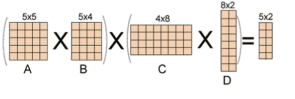
Fig 1: Example of matrix chain multiplication
Solution for Dynamic Programming:
● Take the matrices sequence and divide it into two subsequences.
● Calculate the cheapest way to multiply each subsequence.
● Add all these expenses, as well as the cost of multiplying the two result matrices.
● Do this for each conceivable split position in the series of matrices, and take the lowest of all of them.
The longest here denotes that the subsequence should be the most significant. The term "common" refers to the fact that some of the characters in the two strings are the same. The term "subsequence" refers to the extraction of some characters from a string that is written in ascending order to generate a subsequence.
Let's look at an example to better grasp the subsequence.
Let's say we have the string 'w'.
W1 = abcd
The subsequences that can be made from the aforementioned string are as follows:
Ab
Bd
Ac
Ad
Acd
Bcd
As all the letters in a sub-string are written in increasing order with respect to their place, the above are the subsequences. If we write ca or da, the subsequence will be incorrect since the characters will not appear in increasing order. The total number of possible subsequences is 2n, where n is the number of characters in a string. Because the value of 'n' in the given string is 4, the total number of subsequences is 16.
W2= bcd
We may deduce that bcd is the longest common subsequence by looking at both strings w1 and w2. If the strings are long, finding the subsequence of each and comparing them to discover the longest common subsequence will be impossible.
LCS Problem Statement:
Determine the length of the longest subsequence in each of two sequences. A subsequence is a series of events that occur in the same order but are not necessarily contiguous. Subsequences of "abcdefg" include "abc", "abg", "bdf", "aeg", "acefg", and so on.
To determine the complexity of the brute force method, we must first determine the number of different subsequences of a string of length n, i.e., the number of subsequences with lengths ranging from 1,2,...n-1. Remember from permutation and combination theory that the number of combinations with one element is nC1. nC2 is the number of combinations with two elements, and so on.
nC0 + nC1 + nC2 +... nCn = 2n, as we know. Because we don't examine the subsequence of length 0, a string of length n has 2n-1 different possible subsequences. As a result, the brute force approach's temporal complexity will be O(n * 2n). It's worth noting that determining if a subsequence is shared by both strings requires O(n) time. Dynamic programming can help with this time complexity.
It's a classic computer science problem that's at the heart of diff (a file comparison programme that shows the differences between two files) and has bioinformatics applications.
Examples:
LCS for input Sequences “ABCDGH” and “AEDFHR” is “ADH” of length 3.
LCS for input Sequences “AGGTAB” and “GXTXAYB” is “GTAB” of length 4.
As we know, the nodes in the left subtree have a lower value than the root node, while the nodes in the right subtree have a higher value than the root node in a binary search tree.
We know the key values of each node in the tree, as well as the frequencies of each node in terms of searching, which is the amount of time it takes to find a node. The overall cost of searching a node is determined by the frequency and key-value. In a variety of applications, the cost of searching is a critical element. The cost of searching a node should be lower overall. Because a balanced binary search tree has fewer levels than the BST, the time required to search a node in the BST is longer. The term "optimal binary search tree" refers to a method of lowering the cost of a binary search tree.
Example
If the keys are 10, 20, 30, 40, 50, 60, 70

All of the nodes on the left subtree are smaller than the root node's value, whereas all of the nodes on the right subtree are greater than the root node's value. The greatest time required to search a node is equal to logn times the tree's minimum height.
Now we'll check how many binary search trees we can make with the quantity of keys we have.
For example, the keys are 10, 20, and 30, and the binary search trees that can be generated from these keys are as follows.
The following is the formula for determining the number of trees:

When we utilize the above calculation, we discover that we can make a total of 5 trees.
The cost of looking for an element is determined by the comparisons that must be done. Now we'll figure out what the average time cost of the above binary search trees is.

A total of three comparisons may be made in the tree above. The average number of comparisons is calculated as follows:


The average number of comparisons that can be made in the above tree is:


The average number of comparisons that can be made in the above tree is:


The total number of comparisons in the tree above is three. As a result, the average number of possible comparisons is:


The total number of comparisons in the tree above is three. As a result, the average number of possible comparisons is:

The number of comparisons is lower in the third example since the tree's height is lower, hence it's a balanced binary search tree.
It is a general algorithmic technique
● Backtracking algorithm is used to solve a problem recursively to get a solution incrementally.
● It is used to solve problems when the sequence of objects is chosen from a specified set so that the sequence can satisfy some criteria.
● Backtracking is the systematic method which helps to try out a sequence of decisions until you find out that solution.
● It starts with one smaller piece at a time, if its solution fails to satisfy the constraint then it can be removed at any point of time.
● It searches for any possible combination in order to solve a computational problem.

Fig 2: a - backtracking
However, we usually design our trees from the top down, with the root at the bottom.

Fig 3: Backtracking
Nodes are the building blocks of a tree.

Fig 4: Backtracking
Backtracking is similar to searching a tree for a certain "target" leaf node.
Backtracking is straightforward: we "examine" each node as follows:
To "explore" node N:
1. If N is a goal node, return "success"
2. If N is a leaf node, return "failure"
3. For each child C of N,
Explore C
If C was successful, return "success"
4. Return "failure"
Two constraints:
- Implicit constraint
- Explicit constraint
The backtracking algorithm finds the solution by scanning the solution space for the given problem in a systematic manner. With any bounding function, backtracking is a depth-first search. All backtracking solutions are required to fulfill a complex set of restrictions. Constraints might be stated explicitly or implicitly.
The Explicit Constraint is enforced, which limits each vector element's selection to the supplied set.
Implicit Constraint is ruled, which determines which each of the tuples in the solution space actually satisfy the criterion function.
Application:
- N-queen problem
- Sum of subset
- Graph coloring
- Hamilton problems
Queen problem
Let chess board having N*N cells.
- We need to place N queens in such a way that no queen is attacked by any other queen.
- The queen can attack horizontally, vertically and diagonally. So initially, we are having N*N unattacked cells where we can place the N queens.
Step 1: Place the first queen at a cell (i,j). Hence the unattacked cell is reduced and the number of queens to be placed is N−1.
Step 2: Place the second queen on an unattacked cell that will reduce the no. Of unattacked cells and no. Of queen to be placed become N-2.
The process continues until it satisfies the following condition.
The no. Of unattacked cell become 0
The no of queens to be placed is not 0.
Step 3: As it satisfies the first condition given above then it’s over, we got a final solution.
But if the unattacked cells become 0, then we need to backtrack and remove the last placed queen from its current place and place it in another cell.
This process will be done recursively.
Example:
8-Queen problem
- The eight-queen problem is the problem of placing eight queens on an 8×8 chessboard such that none of them attack one another.
- The eight-queen puzzle has 92 distinct solutions.
- If a solution that differs only by symmetry operation of the board are counted as one puzzle has 12 unique solutions.
Formulation of problem:
- States: any arrangement of 8 queens on board
- Initial state: 0 queens on the board
- Successor function: add a queen on any square
- Goal state: unattacked 8 queens on the board
Steps to be perform:
- Place the first queen in the left upper corner of the table
- Save the attacked position
- Move to the next queen which can only placed on next line
- Search for a valid position. (unattacked position) If there is one go to step 8.
- There is not a valid position for a queen then delete it.
- Move to the previous queen
- Got to step 4
- Place it to the first valid position
- Save the attacked positions
- If the queen processed is the last stop otherwise go to step 3.
Algorithm:
PutQueen(row)
{
For every position col on the same row
If the position col is available
Place the next queen in position col
If(row<8)
putQueen(row+1)
Else success
Remove the queen from positioncol
}
Key takeaway
- Backtracking algorithm is used to solve a problem recursively to get a solution incrementally.
- It is used to solve problems when the sequence of objects is chosen from a specified set so that the sequence can satisfy some criteria.
We must use the Backtracking technique to identify the Hamiltonian Circuit given a graph G = (V, E). We begin our search at any random vertex, such as 'a.' The root of our implicit tree is this vertex 'a.' The first intermediate vertex of the Hamiltonian Cycle to be constructed is the first element of our partial solution. By alphabetical order, the next nearby vertex is chosen.
A dead end is reached when any arbitrary vertices forms a cycle with any vertex other than vertex 'a' at any point. In this situation, we backtrack one step and restart the search by selecting a new vertex and backtracking the partial element; the answer must be removed. If a Hamiltonian Cycle is found, the backtracking search is successful.
Example - Consider the graph G = (V, E) in fig. We must use the Backtracking method to find a Hamiltonian circuit.

To begin, we'll start with vertex 'a,' which will serve as the root of our implicit tree.

Following that, we select the vertex 'b' adjacent to 'a' because it is the first in lexicographical order (b, c, d).

Then, next to 'b,' we select 'c.'

Next, we choose the letter 'd,' which is adjacent to the letter 'c.'

Then we select the letter 'e,' which is adjacent to the letter 'd.'
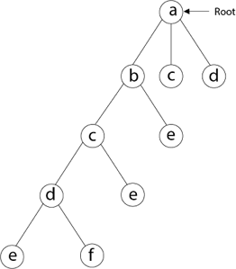
Then, adjacent to 'e,' we select vertex 'f.' D and e are the vertex next to 'f,' but they've already been there. As a result, we reach a dead end and go back a step to delete the vertex 'f' from the partial solution.

The vertices adjacent to 'e' is b, c, d, and f, from which vertex 'f' has already been verified, and b, c, and d have previously been visited, according to backtracking. As a result, we go back one step. The vertex adjacent to d is now e, f, from which e has already been checked, and the vertex adjacent to 'f' is now d and e. We get a dead state if we revisit the 'e' vertex. As a result, we go back one step.
References:
- Analysis and Design of Algorithms: A Beginner's Approach, by Rajesh K. Shukla, Wiley Publications
- “Algorithms, Data Structuresand Problem Solving with C++”, Illustrated Edition by Mark Allen Weiss, Addison-Wesley Publishing Company.
- Data structures and Algorithm Analysis in C, 2nd edition, M.A.Weiss, Pearson
- Data Structures with C, Seymour Lipschutz, Schaum's Outlines, Tata McGraw Hill Education.