Unit - 1
Digital Communication Concept
Let A and B be two events of a sample space Sand let  . Then conditional probability of the event A, given B, denoted by
 is defined by –

Theorem: If the events A and B defined on a sample space S of a random experiment are independent, then

Example1: A factory has two machines A and B making 60% and 40% respectively of the total production. Machine A produces 3% defective items, and B produces 5% defective items. Find the probability that a given defective part came from A.
SOLUTION: We consider the following events:
A: Selected item comes from A.
B: Selected item comes from B.
D: Selected item is defective.
We are looking for  . We know:

Now,

So we need


Since, D is the union of the mutually exclusive events  and
and  (the entire sample space is the union of the mutually exclusive events A and B)


Key Takeaways:
If the events A and B defined on a sample space S of a random experiment are independent, then

A random variable (RV) X is a function from the sample space Ω to the real numbers X:Ω→R
Assuming E⊂RE⊂R we denote the
Event {ω∈Ω:X(ω)∈E}⊂Ωby {X∈E} or just X∈E.
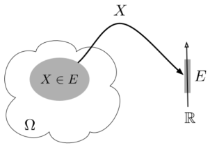
Fig.1: Random variable
Many of the variables dealt with in physics can be expressed as a sum of other variables; often the components of the sum are statistically independent. This section deals with determining the behavior of the sum from the properties of the individual components. First, simple averages are used to find the mean and variance of the sum of statistically independent elements. Next, functions of a random variable are used to examine the probability density of the sum of dependent as well as independent elements. Finally, the Central Limit Theorem is introduced and discussed.
Y = X1 + X2 + . . . + Xn
EY = EX1 + EX2 + . . . + EXn.
The variance of a sum of two random variables is
Var(X1 + X2) = Var(X1) + Var(X2) + 2Cov(X1, X2)


Random processes are classified according to the type of the index variable and classification of the random variables obtained from samples of the random process. The major classification is given below:
Name | Domain of t | Classification of X(t, s) for a fixed t |
Continuous Random Process | All t ∈ [-, ] | Continuous random variable |
Discrete Random Process | All t ∈ [-, ] | Discrete random variable |
Continuous Random Sequence | Countable set : {t1, t2, . . .} | Continuous Random Variable |
Discrete Random Sequence | Countable set : {t1, t2, . . .} | Discrete Random Variable |
A Power Spectral Density (PSD) is the measure of signal's power content versus frequency. A PSD is typically used to characterize broadband random signals. The amplitude of the PSD is normalized by the spectral resolution employed to digitize the signal.
For vibration data, a PSD has amplitude units of g2/Hz. While this unit may not seem intuitive at first, it helps ensure that random data can be overlaid and compared independently of the spectral resolution used to measure the data.
The average power P of a signal x(t) over all time is therefore given by the following time average:

The (cumulative) distribution function (cdf) of a random variable X is defined as the probability of X taking a value less than the argument x:
Fx(x) = P(X ≤ x)
Fx (-) = 0, Fx() = 1
Fx(x1) ≤ Fx (x2) if x1 ≤ x2
The central limit theorem (CLT) is one of the most important results in probability theory.
It states that, under certain conditions, the sum of a large number of random variables is approximately normal.
Here, we state a version of the CLT that applies to i.i.d. Random variables. Suppose that X1, X2 , ... , Xn are i.i.d. Random variables with expected values EXi=μ<∞ and variance Var(Xi)=σ2<∞. Then the sample mean X¯¯=X1+X2+...+Xnn has mean EX¯=μ and variance Var(X¯)=σ2n.
 = μ
= μ
 =
= 
Where,
μ = Population mean
σ = Population standard deviation
μx¯= Sample mean
σx¯ = Sample standard deviation
n = Sample size
How to Apply The Central Limit Theorem (CLT)
Here are the steps that we need in order to apply the CLT:
1.Write the random variable of interest, Y, as the sum of n i.i.d. Random variable Xi's:
Y=X1+X2+...+Xn.
2.Find EY and Var(Y) by noting that
EY=nμ,Var(Y)=nσ2,
Where μ=EXi and σ2=Var(Xi).
3.According to the CLT, conclude that
Y−EY/ √Var(Y)=Y−nμ/ √nσ is approximately standard normal; thus, to find P(y1≤Y≤y2), we can write
P(y1≤Y≤y2)=P(y1−nμ/√nσ≤Y−nμ/√nσ≤y2−nμ/√nσ)
≈Φ(y2−nμ/ √nσ)−Φ(y1−nμ/√nσ).
Q) In a communication system each data packet consists of 1000 bits. Due to the noise, each bit may be received in error with probability 0.1. It is assumed bit errors occur independently. Find the probability that there are more than 120 errors in a certain data packet.
Solution
Let us define Xi as the indicator random variable for the ith bit in the packet. That is, Xi=1 if the ith bit is received in error, and Xi=0 otherwise. Then the Xi's are i.i.d. And Xi∼Bernoulli(p=0.1).
If Y is the total number of bit errors in the packet, we have
Y=X1+X2+...+Xn.
Since Xi∼Bernoulli(p=0.1), we have
EXi=μ=p=0.1,Var(Xi)=σ2=p(1−p)=0.09
Using the CLT, we have
P(Y>120)=P(Y−nμ/ √nσ>120−nμ/√nσ)
=P(Y−nμ/√nσ>120−100/ √90)
≈1−Φ(20/√90)=0.0175
Continuity Correction:
Let us assume that Y∼Binomial(n=20,p=12), and suppose that we are interested in P(8≤Y≤10). We know that a Binomial(n=20,p=12) can be written as the sum of n i.i.d. Bernoulli(p) random variables:
Y=X1+X2+...+Xn.
Since Xi∼Bernoulli(p=12), we have
EXi=μ=p=12,Var(Xi)=σ2=p(1−p)=14.
Thus, we may want to apply the CLT to write
P(8≤Y≤10)=P(8−nμ/√nσ<Y−nμ/√nσ<10−nμ/ √nσ)
=P(8−10/√5 <Y−nμ/ √nσ<10−10/ √5)≈Φ(0)−Φ(−2/√5)=0.3145
Since, here, n=20 is relatively small, we can actually find P(8≤Y≤10) accurately. We have
P(8≤Y≤10)=  pk(1−p)n−k
[(20/8) + (20/9) + (20/10)] (1/2)20
=0.4565
We notice that our approximation is not so good. Part of the error is due to the fact that Y is a discrete random variable and we are using a continuous distribution to find P(8≤Y≤10). Here is a trick to get a better approximation, called continuity correction. Since Y can only take integer values, we can write
P(8≤Y≤10)
=P(7.5<Y<10.5)
=P(7.5−nμ/√nσ<Y−nμ/√nσ<10.5−nμ/√nσ)
=P(7.5−10/√5 <Y−nμ/√nσ<10.5−10/√5)
≈Φ(0.5/√5)−Φ(−2.5/√5)
=0.4567
As we see, using continuity correction, our approximation improved significantly. The continuity correction is particularly useful when we would like to find P(y1≤Y≤y2), where Y is binomial and y1 and y2 are close to each other.
The elements which form a digital communication system is represented by the following block diagram for the ease of understanding.
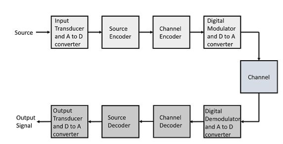
Fig 2 Elements of Digital Communication System
Following are the sections of the digital communication system.
Source
The source can be an analog signal.
Example: A Sound signal
Input Transducer
This is a transducer which takes a physical input and converts it to an electrical signal. This block also consists of an analog to digital converter where a digital signal is needed for further processes.
A digital signal is generally represented by a binary sequence.
Source Encoder
The source encoder compresses the data into minimum number of bits. This process helps in effective utilization of the bandwidth. It removes the redundant bits unnecessary excess bits, i.e. ,zeroes.
Channel Encoder
The channel encoder, does the coding for error correction. During the transmission of the signal, due to the noise in the channel, the signal may get altered and hence to avoid this, the channel encoder adds some redundant bits to the transmitted data. These are the error correcting bits.
Digital Modulator
The signal to be transmitted is modulated here by a carrier. The signal is also converted to analog from the digital sequence, in order to make it travel through the channel or medium.
Channel
The channel or a medium, allows the analog signal to transmit from the transmitter end to the receiver end.
Digital Demodulator
This is the first step at the receiver end. The received signal is demodulated as well as converted again from analog to digital. The signal gets reconstructed here.
Channel Decoder
The channel decoder, after detecting the sequence, does some error corrections. The distortions which might occur during the transmission, are corrected by adding some redundant bits. This addition of bits helps in the complete recovery of the original signal.
Source Decoder
The resultant signal is once again digitized by sampling and quantizing so that the pure digital output is obtained without the loss of information. The source decoder recreates the source output.
Output Transducer
This is the last block which converts the signal into the original physical form, which was at the input of the transmitter. It converts the electrical signal into physical output.
Output Signal
This is the output which is produced after the whole process.
Key takeaway
The channel decoder, after detecting the sequence, does some error corrections. The distortions which might occur during the transmission, are corrected by adding some redundant bits.
In mathematics, particularly linear algebra and numerical analysis, the Gram-Schmidt process is a method for orthogonalizing a set of vectors in an inner product space.
We know that any signal vector can be represented interms of orthogonal basis functions  . Gram-schmidt orthogonalization procedure is the tool to obtain the orthonormal basis function
To derive an expression for 
Suppose we have set of ‘M’ energy signals denoted by 
Starting with  chosen from set arbitrarily the basis function is defined by

Where  is the energy of the signal
  .
.
From question (1), we can write

We know that  for N=1 eq (2) can be written as

From the above equation (3) we obtain  and
and  has unit energy.
Next, using the signal  we define the co-efficient
Let  be a new intermediate function which is given as
The function is orthogonal to  over the interval 0 to T.
The second function, which is given as

 is the energy of

a) To prove that  has unit energy
Energy of  will be

We know that 


b) To prove that  and
and  are orthogonal
Consider 
Substitute the values of  and
and  in the above equation. i.e
 and
and 


Substitute 


We know that


From the given equation there is a product of two terms  and
and  . But the two symbols are not present at a time. Hence the product of
  and
and  . Hence the product of
  and
and  i.e.,
i.e.,  and hence the integration terms in RHS will be zero. Ie
 . Thus, the noo basis function are orthonormal.
Generalized equation for orthonormal basis functions
The generalised equation for orthonormal basis function can be written by considering the following equation i.e.

Where is given by the generalized equation
Note
 are ready taken consideration.
Where the coefficients

For  the
the  redues to
Given the  we may define the set of ban’s function

Which form an orthogonal set. The dimension ‘N’ is less than or equal to the number of given signals, M depending on one of N0 possibilities.
- The signals
 form a linearly independent set, in which case N=M.
 - The signals
 are not linearly independent.
Problem-1
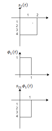
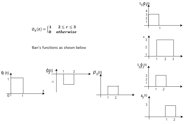
Using the gram-schmidt orthogonalization procedure, find a set of orthonormal ban’s functions represent the tree signals  as shown in figure.

Solution
All the three signals  are not linear combination of each other hence they are linearly independent. Hence, we require three ban’s function.
To obtain 
Energy of 


To obtain 


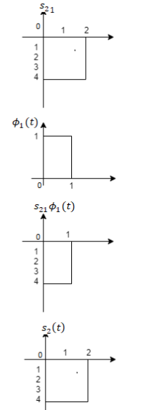
To obtain 


Problem-2
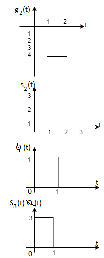
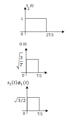
Consider the signals  and
and as given below. Find an orthonormal basis for phase set of signals using Grammar schimdt orthogonalisation procedure.
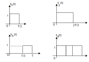
Fig 3. Sketch of  and
and 
Solution:
From the above figures  . This means all four signals are not linearly independent. Gram-schmidt orthogonalisation procedure is carried out for a subset which is linearly independent. Here
  are linearly independent. Hence, we will determine orthonormal.
To obtain 
Energy of  is
is 


We know that


To obtain 


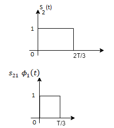
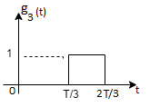
From the above figure the intermediate function can be defined as

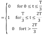

Energy of  will be


Now


To obtain 
We know that the generalized equation for gram-schmitt procedure

With N=3


We know that


Since, there is no overlap between  and
and 

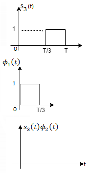


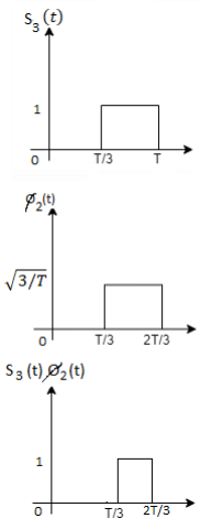
Here 


We know that


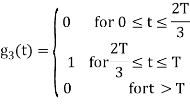

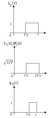


Figure below shows orthonormal basis function

Problem 3:
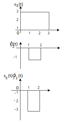
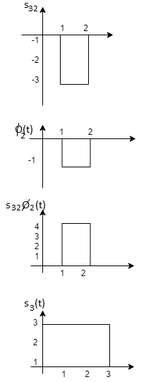
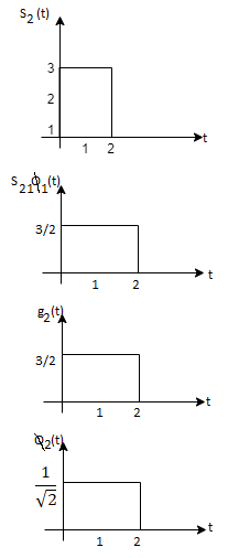
Three signals  are shown in fig. Apply Gram-schmidt procedure to obtain an orthonormal basis for the signals. Express signals
  in terms of orthonormal basis function.

Solution
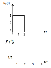
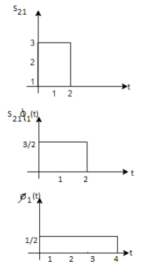
i) To obtain orthonormal basis function
Here 
Hence, we will obtain basis solution for  and
and  only.
only.
To obtain 
Energy of  is
is 


We know that

To obtain 






As in the case of vectors, we may develop a parallel treatment for a set of signals.
The inner product of two generally complex-valued signals x1(t) and x2(t) is denoted by <x1(t), x2(t)> and defined by

The signals are orthogonal if their inner product is zero. The norm of a signal is defined as

Where  x is the energy in x(t). A set of m signal is orthonormal if they are orthogonal and their norms are all unity.
The Gram-Schmidt orthogonalization procedure can be used to construct a set of orthonormal waveforms from a set of finite energy signal waveforms: xi(t), 1 ≤ i ≤ m.
Once we have constructed the set of, say k, orthonormal waveforms {φk(t)}, we can express the signals {xi(t)} as linear combinations of the φk(t). Thus, we may write

Based on the above expression, each signal may be represented by the vector
x (i) = (xi,1, xi,2, . . . , xi,K ) T
Or, equivalently, as a point in the N-dimensional (in general, complex) signal space.
A set of M signals {xi(t)} can be represented by a set of M vectors {x (i)} in the N-dimensional space. The corresponding set of vectors is called the signal space representation, or constellation, of {xi(t)}.
• If the original signals are real, then the corresponding vector representations are in RK; and if the signals are complex, then the vector representations are in CK.
• Figure demonstrates the process of obtaining the vector equivalent from a signal (signal-to-vector mapping) and vice versa (vector-to signal mapping).
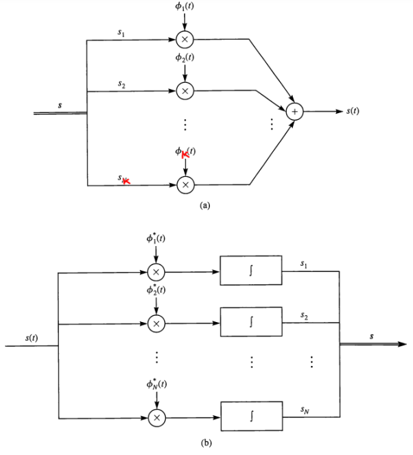
Fig 4. Vector to signal (a), and signal to vector (b) mappings
Geometric representation of signals can provide a compact characterization of signals and can simplify analysis of their performance as modulation signals. Orthonormal bases are essential in geometry. Let {s1 (t), s2 (t), . . . , sM (t)} be a set of signals.
ψ1(t) = s1(t)/E1 where E1 = 
s21 = < s2, ψ1 >=  and ψ2(t) = 1/
 2(s2(t) – s21(t) – s21ψ1)
 2 =
2 = 
ψk(t) = 1/ 2 ( sk(t) –
  )
)
 k =
k = 
sm(t) = 
The process continues until all of the M signals are exhausted. The results are N orthogonal signals with unit energy, {ψ1 (t), ψ2 (t), . . . , ψN (t)}. If the signals {s1 (t), . . . , sM (t)} are linearly independent, then N = M.
m ∈ {1, 2, . . . , M}
The M signals can be represented as
smn =< sm, ψn > and Em = 

The analysis for SNRI and SNRO assumes perfectly white noise j (t) for simplicity. Note that a white noise j(t) has infinite power such that j (t) and c(t)j(t) will have the same PSD


Fig 5. PDF Comparison
P(Error) = (0-  /σ) = (0 -
  /
/  ) = ( -
  )
)
As discussed earlier that a noise interference may lead to wrong decision at the receiver end. As a matter of fact, the probability of error denoted by Pe is a good measure of performance of the detector.
We know that the output of the integrator is expressed as
y(t) = x0(t) + n0(t)
For the positive pulse of amplitude A, x0(t) is given as
x0(t)= or x(t) =A
Similarly, For the input pulse of amplitude -A, x0(t)is given as
x0(t)= or x(t)=-A
Therefore, the output y(t) may be written as
x(t)= or x(t)=A (1)
Similarly, y(t)= or x(t)=-A (2)
Let us consider that x(t)=-A. Further if noise n0(t)is greater than, then the output y(t) would be positive according to equation (2). After that the receiver will decide in favour of symbol +A, which is wrong decision. This means that an error is introduced.
Similarly, let us consider that x(t) = +A If noise n0(t)>-then, the output y(t) will be negative according to equation (1). This leads to decision in favour of –A, which is erroneous. Based on the above discussion we can make conclusions about probability of error in the form of a below table.
Probability of error in integrate and dump filter receiver
S.No | Input x(t) | Value of n0(t) For error in the output | The probability of error Pe |
1 | -A | An error will be introduced if n0(t)> | In this case the probability of error may be obtained by calculating probability that n0(t)> |
2 | +A | An error will be introduced if n0(t)< | In this case the probability of error may be obtained by calculating probability that n0(t)< |
In other terms, the inner product is a correlation

But we want to build a receiver that does the minimum amount of calculation. If si(t) are non-orthogonal, then we can reduce the amount of correlation (and thus multiplication and addition) done in the receiver by instead, correlating with the basis functions, {φk(t)} N k=1. Correlation with the basis functions gives

x = [x1, x2, . . . , xN]T
Now that we’ve done these N correlations (inner products), we can compute the estimate of the received signal as

r(t) = bsi(t) + n(t)
n(t) = 0 and b = 1
x = ai
Where ai is the signal space vector for si(t).
Our signal set can be represented by the orthonormal basis functions, . Correlation with the basis functions gives
For k = 0 . . . K − 1. We denote vectors:
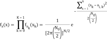
Hopefully, x and ai should be close since i was actually sent. In general, the pdf of x is multivariate Gaussian with each component xk independent, because
- xk = ai,k + nk
- ai,k is a deterministic constant
- The {nk} are i.i.d. Gaussian.
The joint pdf of x is
If a filter produces an output in such a way that it maximizes the ratio of output peak power to mean noise power in its frequency response, then that filter is called Matched filter.

Fig 6: Matched filter
Frequency Response Function of Matched Filter
The frequency response of the Matched filter will be proportional to the complex conjugate of the input signal’s spectrum. Mathematically, we can write the expression for frequency response function, H(f) of the Matched filter as −
H(f)=GaS∗(f)e−j2πft1 ………..1
Where,
Ga is the maximum gain of the Matched filter
S(f) is the Fourier transform of the input signal, s(t)
S∗(f) is the complex conjugate of S(f)
t1 is the time instant at which the signal observed to be maximum
In general, the value of Ga is considered as one. We will get the following equation by substituting Ga=1in Equation 1.
H(f)=S∗(f)e−j2πft1 ……..2
The frequency response function, H(f) of the Matched filter is having the magnitude of S∗(f)and phase angle of e−j2πft1, which varies uniformly with frequency.
Impulse Response of Matched Filter
In time domain, we will get the output, h(t) of Matched filter receiver by applying the inverse Fourier transform of the frequency response function, H(f).
h(t) =  .….3
.….3
Substitute, Equation 1 in Equation 3.
h(t) = 
⇒ h(t) =  ………4
………4
We know the following relation.
S∗(f)=S(−f) ……..5
Substitute, Equation 5 in Equation 4.
h(t) = 
h(t) = 
h(t) = Gas(t1 – t)
In general, the value of Ga is considered as one. We will get the following equation by substituting Ga=1.
h(t)=s(t1−t)
The above equation proves that the impulse response of Matched filter is the mirror image of the received signal about a time instant t1. The following figures illustrate this concept.

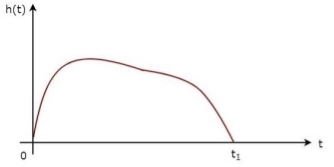
Fig 7: Impulse response of Matched filter
The received signal, s(t) and the impulse response, h(t) of the matched filter corresponding to the signal, s(t) are shown in the above figures.
Key Takeaways:
The frequency response function, H(f) of the Matched filter as −
H(f)=GaS∗(f)e−j2πft1 ………..1
Where,
Ga is the maximum gain of the Matched filter
S(f) is the Fourier transform of the input signal, s(t)
S∗(f) is the complex conjugate of S(f)
t1 is the time instant at which the signal observed to be maximum
Impulse response,h(t)=s(t1 −t)
References:
1. Lathi B.P. - Modern Digital and Analog communications systems - PRISM Indian Ed.
2. Digital Communication: J.S.Chitode
3. Digital Communication (Fundamentals & applications): Bernard Scalr
4. Introduction to Error Control Codes: Salvatore Gravano
5. OFDM For wireless communication systems: Ramjee Prasad
6. Modern Communication systems (Principles and application): Leon W. Couch II (PHI)
7. Error Control Coding: Shu Lin & Daniel J.Costello
Unit - 1
Digital Communication Concept
Unit - 1
Digital Communication Concept
Unit - 1
Digital Communication Concept
Let A and B be two events of a sample space Sand let  . Then conditional probability of the event A, given B, denoted by
 is defined by –

Theorem: If the events A and B defined on a sample space S of a random experiment are independent, then

Example1: A factory has two machines A and B making 60% and 40% respectively of the total production. Machine A produces 3% defective items, and B produces 5% defective items. Find the probability that a given defective part came from A.
SOLUTION: We consider the following events:
A: Selected item comes from A.
B: Selected item comes from B.
D: Selected item is defective.
We are looking for  . We know:

Now,

So we need


Since, D is the union of the mutually exclusive events  and
and  (the entire sample space is the union of the mutually exclusive events A and B)


Key Takeaways:
If the events A and B defined on a sample space S of a random experiment are independent, then

A random variable (RV) X is a function from the sample space Ω to the real numbers X:Ω→R
Assuming E⊂RE⊂R we denote the
Event {ω∈Ω:X(ω)∈E}⊂Ωby {X∈E} or just X∈E.

Fig.1: Random variable
Many of the variables dealt with in physics can be expressed as a sum of other variables; often the components of the sum are statistically independent. This section deals with determining the behavior of the sum from the properties of the individual components. First, simple averages are used to find the mean and variance of the sum of statistically independent elements. Next, functions of a random variable are used to examine the probability density of the sum of dependent as well as independent elements. Finally, the Central Limit Theorem is introduced and discussed.
Y = X1 + X2 + . . . + Xn
EY = EX1 + EX2 + . . . + EXn.
The variance of a sum of two random variables is
Var(X1 + X2) = Var(X1) + Var(X2) + 2Cov(X1, X2)


Random processes are classified according to the type of the index variable and classification of the random variables obtained from samples of the random process. The major classification is given below:
Name | Domain of t | Classification of X(t, s) for a fixed t |
Continuous Random Process | All t ∈ [-, ] | Continuous random variable |
Discrete Random Process | All t ∈ [-, ] | Discrete random variable |
Continuous Random Sequence | Countable set : {t1, t2, . . .} | Continuous Random Variable |
Discrete Random Sequence | Countable set : {t1, t2, . . .} | Discrete Random Variable |
A Power Spectral Density (PSD) is the measure of signal's power content versus frequency. A PSD is typically used to characterize broadband random signals. The amplitude of the PSD is normalized by the spectral resolution employed to digitize the signal.
For vibration data, a PSD has amplitude units of g2/Hz. While this unit may not seem intuitive at first, it helps ensure that random data can be overlaid and compared independently of the spectral resolution used to measure the data.
The average power P of a signal x(t) over all time is therefore given by the following time average:

The (cumulative) distribution function (cdf) of a random variable X is defined as the probability of X taking a value less than the argument x:
Fx(x) = P(X ≤ x)
Fx (-) = 0, Fx() = 1
Fx(x1) ≤ Fx (x2) if x1 ≤ x2
The central limit theorem (CLT) is one of the most important results in probability theory.
It states that, under certain conditions, the sum of a large number of random variables is approximately normal.
Here, we state a version of the CLT that applies to i.i.d. Random variables. Suppose that X1, X2 , ... , Xn are i.i.d. Random variables with expected values EXi=μ<∞ and variance Var(Xi)=σ2<∞. Then the sample mean X¯¯=X1+X2+...+Xnn has mean EX¯=μ and variance Var(X¯)=σ2n.
 = μ
= μ
 =
= 
Where,
μ = Population mean
σ = Population standard deviation
μx¯= Sample mean
σx¯ = Sample standard deviation
n = Sample size
How to Apply The Central Limit Theorem (CLT)
Here are the steps that we need in order to apply the CLT:
1.Write the random variable of interest, Y, as the sum of n i.i.d. Random variable Xi's:
Y=X1+X2+...+Xn.
2.Find EY and Var(Y) by noting that
EY=nμ,Var(Y)=nσ2,
Where μ=EXi and σ2=Var(Xi).
3.According to the CLT, conclude that
Y−EY/ √Var(Y)=Y−nμ/ √nσ is approximately standard normal; thus, to find P(y1≤Y≤y2), we can write
P(y1≤Y≤y2)=P(y1−nμ/√nσ≤Y−nμ/√nσ≤y2−nμ/√nσ)
≈Φ(y2−nμ/ √nσ)−Φ(y1−nμ/√nσ).
Q) In a communication system each data packet consists of 1000 bits. Due to the noise, each bit may be received in error with probability 0.1. It is assumed bit errors occur independently. Find the probability that there are more than 120 errors in a certain data packet.
Solution
Let us define Xi as the indicator random variable for the ith bit in the packet. That is, Xi=1 if the ith bit is received in error, and Xi=0 otherwise. Then the Xi's are i.i.d. And Xi∼Bernoulli(p=0.1).
If Y is the total number of bit errors in the packet, we have
Y=X1+X2+...+Xn.
Since Xi∼Bernoulli(p=0.1), we have
EXi=μ=p=0.1,Var(Xi)=σ2=p(1−p)=0.09
Using the CLT, we have
P(Y>120)=P(Y−nμ/ √nσ>120−nμ/√nσ)
=P(Y−nμ/√nσ>120−100/ √90)
≈1−Φ(20/√90)=0.0175
Continuity Correction:
Let us assume that Y∼Binomial(n=20,p=12), and suppose that we are interested in P(8≤Y≤10). We know that a Binomial(n=20,p=12) can be written as the sum of n i.i.d. Bernoulli(p) random variables:
Y=X1+X2+...+Xn.
Since Xi∼Bernoulli(p=12), we have
EXi=μ=p=12,Var(Xi)=σ2=p(1−p)=14.
Thus, we may want to apply the CLT to write
P(8≤Y≤10)=P(8−nμ/√nσ<Y−nμ/√nσ<10−nμ/ √nσ)
=P(8−10/√5 <Y−nμ/ √nσ<10−10/ √5)≈Φ(0)−Φ(−2/√5)=0.3145
Since, here, n=20 is relatively small, we can actually find P(8≤Y≤10) accurately. We have
P(8≤Y≤10)=  pk(1−p)n−k
[(20/8) + (20/9) + (20/10)] (1/2)20
=0.4565
We notice that our approximation is not so good. Part of the error is due to the fact that Y is a discrete random variable and we are using a continuous distribution to find P(8≤Y≤10). Here is a trick to get a better approximation, called continuity correction. Since Y can only take integer values, we can write
P(8≤Y≤10)
=P(7.5<Y<10.5)
=P(7.5−nμ/√nσ<Y−nμ/√nσ<10.5−nμ/√nσ)
=P(7.5−10/√5 <Y−nμ/√nσ<10.5−10/√5)
≈Φ(0.5/√5)−Φ(−2.5/√5)
=0.4567
As we see, using continuity correction, our approximation improved significantly. The continuity correction is particularly useful when we would like to find P(y1≤Y≤y2), where Y is binomial and y1 and y2 are close to each other.
The elements which form a digital communication system is represented by the following block diagram for the ease of understanding.

Fig 2 Elements of Digital Communication System
Following are the sections of the digital communication system.
Source
The source can be an analog signal.
Example: A Sound signal
Input Transducer
This is a transducer which takes a physical input and converts it to an electrical signal. This block also consists of an analog to digital converter where a digital signal is needed for further processes.
A digital signal is generally represented by a binary sequence.
Source Encoder
The source encoder compresses the data into minimum number of bits. This process helps in effective utilization of the bandwidth. It removes the redundant bits unnecessary excess bits, i.e. ,zeroes.
Channel Encoder
The channel encoder, does the coding for error correction. During the transmission of the signal, due to the noise in the channel, the signal may get altered and hence to avoid this, the channel encoder adds some redundant bits to the transmitted data. These are the error correcting bits.
Digital Modulator
The signal to be transmitted is modulated here by a carrier. The signal is also converted to analog from the digital sequence, in order to make it travel through the channel or medium.
Channel
The channel or a medium, allows the analog signal to transmit from the transmitter end to the receiver end.
Digital Demodulator
This is the first step at the receiver end. The received signal is demodulated as well as converted again from analog to digital. The signal gets reconstructed here.
Channel Decoder
The channel decoder, after detecting the sequence, does some error corrections. The distortions which might occur during the transmission, are corrected by adding some redundant bits. This addition of bits helps in the complete recovery of the original signal.
Source Decoder
The resultant signal is once again digitized by sampling and quantizing so that the pure digital output is obtained without the loss of information. The source decoder recreates the source output.
Output Transducer
This is the last block which converts the signal into the original physical form, which was at the input of the transmitter. It converts the electrical signal into physical output.
Output Signal
This is the output which is produced after the whole process.
Key takeaway
The channel decoder, after detecting the sequence, does some error corrections. The distortions which might occur during the transmission, are corrected by adding some redundant bits.
In mathematics, particularly linear algebra and numerical analysis, the Gram-Schmidt process is a method for orthogonalizing a set of vectors in an inner product space.
We know that any signal vector can be represented interms of orthogonal basis functions  . Gram-schmidt orthogonalization procedure is the tool to obtain the orthonormal basis function
To derive an expression for 
Suppose we have set of ‘M’ energy signals denoted by 
Starting with  chosen from set arbitrarily the basis function is defined by

Where  is the energy of the signal
  .
.
From question (1), we can write

We know that  for N=1 eq (2) can be written as

From the above equation (3) we obtain  and
and  has unit energy.
Next, using the signal  we define the co-efficient
Let  be a new intermediate function which is given as
The function is orthogonal to  over the interval 0 to T.
The second function, which is given as

 is the energy of

a) To prove that  has unit energy
Energy of  will be

We know that 


b) To prove that  and
and  are orthogonal
Consider 
Substitute the values of  and
and  in the above equation. i.e
 and
and 


Substitute 


We know that


From the given equation there is a product of two terms  and
and  . But the two symbols are not present at a time. Hence the product of
  and
and  . Hence the product of
  and
and  i.e.,
i.e.,  and hence the integration terms in RHS will be zero. Ie
 . Thus, the noo basis function are orthonormal.
Generalized equation for orthonormal basis functions
The generalised equation for orthonormal basis function can be written by considering the following equation i.e.

Where is given by the generalized equation
Note
 are ready taken consideration.
Where the coefficients

For  the
the  redues to
Given the  we may define the set of ban’s function

Which form an orthogonal set. The dimension ‘N’ is less than or equal to the number of given signals, M depending on one of N0 possibilities.
- The signals
 form a linearly independent set, in which case N=M.
 - The signals
 are not linearly independent.
Problem-1
Using the gram-schmidt orthogonalization procedure, find a set of orthonormal ban’s functions represent the tree signals  as shown in figure.
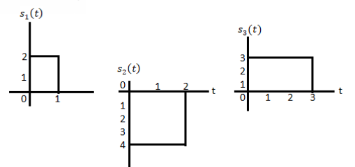
Solution
All the three signals  are not linear combination of each other hence they are linearly independent. Hence, we require three ban’s function.
To obtain 
Energy of 


To obtain 




To obtain 





Problem-2
Consider the signals  and
and as given below. Find an orthonormal basis for phase set of signals using Grammar schimdt orthogonalisation procedure.

Fig 3. Sketch of  and
and 
Solution:
From the above figures  . This means all four signals are not linearly independent. Gram-schmidt orthogonalisation procedure is carried out for a subset which is linearly independent. Here
  are linearly independent. Hence, we will determine orthonormal.
To obtain 
Energy of  is
is 


We know that


To obtain 




From the above figure the intermediate function can be defined as


Energy of  will be


Now


To obtain 
We know that the generalized equation for gram-schmitt procedure

With N=3


We know that


Since, there is no overlap between  and
and 


Here 


We know that


Figure below shows orthonormal basis function

Problem 3:
Three signals  are shown in fig. Apply Gram-schmidt procedure to obtain an orthonormal basis for the signals. Express signals
  in terms of orthonormal basis function.

Solution
i) To obtain orthonormal basis function
Here 
Hence, we will obtain basis solution for  and
and  only.
only.
To obtain 
Energy of  is
is 


We know that

To obtain 


As in the case of vectors, we may develop a parallel treatment for a set of signals.
The inner product of two generally complex-valued signals x1(t) and x2(t) is denoted by <x1(t), x2(t)> and defined by

The signals are orthogonal if their inner product is zero. The norm of a signal is defined as

Where  x is the energy in x(t). A set of m signal is orthonormal if they are orthogonal and their norms are all unity.
The Gram-Schmidt orthogonalization procedure can be used to construct a set of orthonormal waveforms from a set of finite energy signal waveforms: xi(t), 1 ≤ i ≤ m.
Once we have constructed the set of, say k, orthonormal waveforms {φk(t)}, we can express the signals {xi(t)} as linear combinations of the φk(t). Thus, we may write

Based on the above expression, each signal may be represented by the vector
x (i) = (xi,1, xi,2, . . . , xi,K ) T
Or, equivalently, as a point in the N-dimensional (in general, complex) signal space.
A set of M signals {xi(t)} can be represented by a set of M vectors {x (i)} in the N-dimensional space. The corresponding set of vectors is called the signal space representation, or constellation, of {xi(t)}.
• If the original signals are real, then the corresponding vector representations are in RK; and if the signals are complex, then the vector representations are in CK.
• Figure demonstrates the process of obtaining the vector equivalent from a signal (signal-to-vector mapping) and vice versa (vector-to signal mapping).

Fig 4. Vector to signal (a), and signal to vector (b) mappings
Geometric representation of signals can provide a compact characterization of signals and can simplify analysis of their performance as modulation signals. Orthonormal bases are essential in geometry. Let {s1 (t), s2 (t), . . . , sM (t)} be a set of signals.
ψ1(t) = s1(t)/E1 where E1 = 
s21 = < s2, ψ1 >=  and ψ2(t) = 1/
 2(s2(t) – s21(t) – s21ψ1)
 2 =
2 = 
ψk(t) = 1/ 2 ( sk(t) –
  )
)
 k =
k = 
sm(t) = 
The process continues until all of the M signals are exhausted. The results are N orthogonal signals with unit energy, {ψ1 (t), ψ2 (t), . . . , ψN (t)}. If the signals {s1 (t), . . . , sM (t)} are linearly independent, then N = M.
m ∈ {1, 2, . . . , M}
The M signals can be represented as
smn =< sm, ψn > and Em = 

The analysis for SNRI and SNRO assumes perfectly white noise j (t) for simplicity. Note that a white noise j(t) has infinite power such that j (t) and c(t)j(t) will have the same PSD

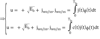
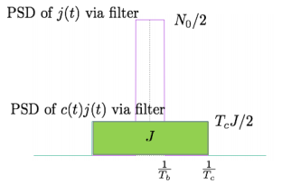
Fig 5. PDF Comparison
P(Error) = (0-  /σ) = (0 -
  /
/  ) = ( -
  )
)
As discussed earlier that a noise interference may lead to wrong decision at the receiver end. As a matter of fact, the probability of error denoted by Pe is a good measure of performance of the detector.
We know that the output of the integrator is expressed as
y(t) = x0(t) + n0(t)
For the positive pulse of amplitude A, x0(t) is given as
x0(t)= or x(t) =A
Similarly, For the input pulse of amplitude -A, x0(t)is given as
x0(t)= or x(t)=-A
Therefore, the output y(t) may be written as
x(t)= or x(t)=A (1)
Similarly, y(t)= or x(t)=-A (2)
Let us consider that x(t)=-A. Further if noise n0(t)is greater than, then the output y(t) would be positive according to equation (2). After that the receiver will decide in favour of symbol +A, which is wrong decision. This means that an error is introduced.
Similarly, let us consider that x(t) = +A If noise n0(t)>-then, the output y(t) will be negative according to equation (1). This leads to decision in favour of –A, which is erroneous. Based on the above discussion we can make conclusions about probability of error in the form of a below table.
Probability of error in integrate and dump filter receiver
S.No | Input x(t) | Value of n0(t) For error in the output | The probability of error Pe |
1 | -A | An error will be introduced if n0(t)> | In this case the probability of error may be obtained by calculating probability that n0(t)> |
2 | +A | An error will be introduced if n0(t)< | In this case the probability of error may be obtained by calculating probability that n0(t)< |
In other terms, the inner product is a correlation

But we want to build a receiver that does the minimum amount of calculation. If si(t) are non-orthogonal, then we can reduce the amount of correlation (and thus multiplication and addition) done in the receiver by instead, correlating with the basis functions, {φk(t)} N k=1. Correlation with the basis functions gives

x = [x1, x2, . . . , xN]T
Now that we’ve done these N correlations (inner products), we can compute the estimate of the received signal as

r(t) = bsi(t) + n(t)
n(t) = 0 and b = 1
x = ai
Where ai is the signal space vector for si(t).
Our signal set can be represented by the orthonormal basis functions, . Correlation with the basis functions gives
For k = 0 . . . K − 1. We denote vectors:
Hopefully, x and ai should be close since i was actually sent. In general, the pdf of x is multivariate Gaussian with each component xk independent, because
- xk = ai,k + nk
- ai,k is a deterministic constant
- The {nk} are i.i.d. Gaussian.
The joint pdf of x is

If a filter produces an output in such a way that it maximizes the ratio of output peak power to mean noise power in its frequency response, then that filter is called Matched filter.

Fig 6: Matched filter
Frequency Response Function of Matched Filter
The frequency response of the Matched filter will be proportional to the complex conjugate of the input signal’s spectrum. Mathematically, we can write the expression for frequency response function, H(f) of the Matched filter as −
H(f)=GaS∗(f)e−j2πft1 ………..1
Where,
Ga is the maximum gain of the Matched filter
S(f) is the Fourier transform of the input signal, s(t)
S∗(f) is the complex conjugate of S(f)
t1 is the time instant at which the signal observed to be maximum
In general, the value of Ga is considered as one. We will get the following equation by substituting Ga=1in Equation 1.
H(f)=S∗(f)e−j2πft1 ……..2
The frequency response function, H(f) of the Matched filter is having the magnitude of S∗(f)and phase angle of e−j2πft1, which varies uniformly with frequency.
Impulse Response of Matched Filter
In time domain, we will get the output, h(t) of Matched filter receiver by applying the inverse Fourier transform of the frequency response function, H(f).
h(t) =  .….3
.….3
Substitute, Equation 1 in Equation 3.
h(t) = 
⇒ h(t) =  ………4
………4
We know the following relation.
S∗(f)=S(−f) ……..5
Substitute, Equation 5 in Equation 4.
h(t) = 
h(t) = 
h(t) = Gas(t1 – t)
In general, the value of Ga is considered as one. We will get the following equation by substituting Ga=1.
h(t)=s(t1−t)
The above equation proves that the impulse response of Matched filter is the mirror image of the received signal about a time instant t1. The following figures illustrate this concept.
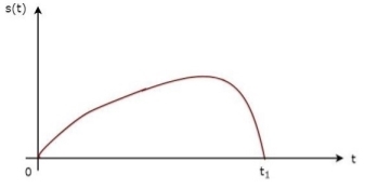

Fig 7: Impulse response of Matched filter
The received signal, s(t) and the impulse response, h(t) of the matched filter corresponding to the signal, s(t) are shown in the above figures.
Key Takeaways:
The frequency response function, H(f) of the Matched filter as −
H(f)=GaS∗(f)e−j2πft1 ………..1
Where,
Ga is the maximum gain of the Matched filter
S(f) is the Fourier transform of the input signal, s(t)
S∗(f) is the complex conjugate of S(f)
t1 is the time instant at which the signal observed to be maximum
Impulse response,h(t)=s(t1 −t)
References:
1. Lathi B.P. - Modern Digital and Analog communications systems - PRISM Indian Ed.
2. Digital Communication: J.S.Chitode
3. Digital Communication (Fundamentals & applications): Bernard Scalr
4. Introduction to Error Control Codes: Salvatore Gravano
5. OFDM For wireless communication systems: Ramjee Prasad
6. Modern Communication systems (Principles and application): Leon W. Couch II (PHI)
7. Error Control Coding: Shu Lin & Daniel J.Costello