Unit - 5
Channel Coding (PART-II)
Code trellis representation
- Code trellis is the more compact representation of the code tree. In the code tree there are four states (or nodes). Every state goes to some other state depending upon the input message bit.
- Code trellis represents the single and unique diagram for such steady state transitions. The Figure below shows the code trellis diagram.
- The nodes on the left denote four possible current states and those on the right represents next state. The solid transition line represents for input message m0 = 0 and dashed line represents input message m0 = 1.
- Along with each transition line, the encoder output x1 x2 is represented during that transition.

Fig: Code Trellis
Advantages of convolutional codes
- The convolutional codes operate on smaller blocks of data. Hence decoding delay is small.
- The storage hardware required is less.
Disadvantages of convolutional codes
- Due to complexity, the convolutional codes are difficult to analyze.
- These codes are not developed much as compared to block codes.
The use of a good code with random-like properties is basic to turbo coding. In the first successful implementation of turbo codes11, Berrouet al. Achieved this design objective by using concatenated codes. The original idea of concatenated codes was conceived by Forney (1966). To be more specific, concatenated codes can be of two types: parallel or serial. The type of concatenated codes used by Berrou et al. Was of the parallel type, which is discussed in this section

Fig: Block diagram of turbo encoder of the parallel type.
Figure above depicts the most basic form of a turbo code generator that consists of two constituent systematic encoders, which are concatenated by means of an interleaver. The interleaver is an input–output mapping device that permutes the ordering of a sequence of symbols from a fixed alphabet in a completely deterministic manner; that is, it takes the symbols at the input and produces identical symbols at the output but in a different temporal order. Turbo codes use a pseudo-random interleaver, which operates only on the systematic (i.e., message) bits. The size of the interleaver used in turbo codes is typically very large, on the order of several thousand bits. There are two reasons for the use of an interleaver in a turbo code:
1. The interleaver ties together errors that are easily made in one half of the turbo code to errors that are exceptionally unlikely to occur in the other half; this is indeed one reason why the turbo code performs better than a traditional code.
2. The interleaver provides robust performance with respect to mismatched decoding, a problem that arises when the channel statistics are not known or have been incorrectly specified.
Ordinarily, but not necessarily, the same code is used for both constituent encoders in Figure above. The constituent codes recommended for turbo codes are short constraint length RSC codes. The reason for making the convolutional codes recursive (i.e., feeding one or more of the tap outputs in the shift register back to the input) is to make the internal state of the shift register depend on past outputs. This affects the behavior of the error patterns, with the result that a better performance of the overall coding strategy is attained.
Two-State Turbo Encoder Figure below shows the block diagram of a specific turbo encoder using an identical pair of two-state RSC constituent encoders. The generator matrix of each constituent encoder is given by
G(D)= (1, 1/1+D)
The input sequence of bits has length, made up of three message bits and one termination bit. The input vector is given by
m= m0 m1 m2 m3

Fig: Two-state turbo encoder for Example
The parity-check vector produced by the first constituent encoder is given by
b(1) = (b0(1), b1(1), b2(1) b3(1))
Similarly, the parity-check vector produced by the second constituent encoder is given by
b(2) = (b0(2), b1(2), b2(2) b3(2))
The transmitted code vector is therefore defined by
c = (c(0), c(1), c(2))
With the convolutional code being systematic, we thus have
c(0) = m
As for the remaining two sub-vectors constituting the code vector c, they are defined by c(1) = b(1) and c(2) = b(2).
The transmitted code vector c is therefore made up of 12 bits. However, recalling that the termination bit m3 is not a message bit, it follows that the code rate of the turbo code
R=3/12=1/4
Turbo Decoder
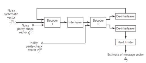
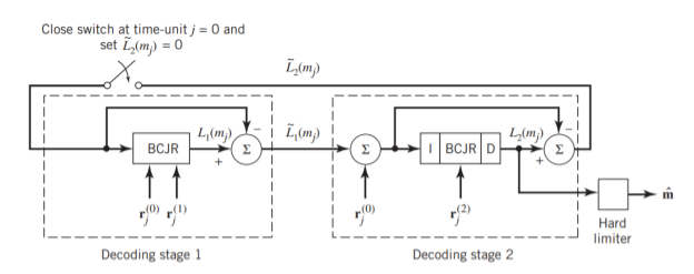
Figure 11(a) below shows the block diagram of the two-stage turbo decoder. The decoder operates on noisy versions of the systematic bits and the two sets of parity-check bits in two decoding stages to produce an estimate of the original message bits. A distinctive feature of the turbo decoder that is immediately apparent from the block diagram of Figure11(a) is the use of feedback, manifesting itself in producing extrinsic information from one decoder to the next in an iterative manner. In a way, this decoding process is analogous to the feedback of exhaust gases experienced in a turbo-charged engine; indeed, turbo codes derive their name from this analogy. In other words, the term “turbo” in turbo codes has more to do with the decoding rather than the encoding process. In operational terms, the turbo encoder in Figure11(a) operates on noisy versions of the following inputs, obtained by demultiplexing the channel output, rj
- Systematic (i.e., message) bits, denoted by rj(0)
- Parity-check bits corresponding to encoder 1 in Figure encoder, denoted by rj(1)
- Parity-check bits corresponding to encoder 2 in Figure encoder, denoted by rj(2)
The net result of the decoding algorithm, given the received vector rj, is an estimate of the original message vector, namely, which is delivered at the decoder output to the user. Another important point to note in the turbo decoder of Figure (a) is the way in which the interleaver and de-interleaver are positioned inside the feedback loop. Bearing in mind the fact that the definition of extrinsic information requires the use of intrinsic information, we see that decoder 1 operates on three inputs:
- The noisy systematic (i.e., original message) bits,
- The noisy parity-check bits due to encoder 1, and
- De-interleaved extrinsic information computed by decoder 2
(a)
(b)
Fig: (a) Block diagram of turbo decoder. (b) Extrinsic form of turbo decoder, where I stand for interleaver, D for deinterleaver, and BCJR for BCJR for BCJR algorithm for log-MAP decoding.
In a complementary manner, decoder 2 operates on two inputs of its own:
- The noisy parity-check bits due to encoder 2 and
- The interleaved version of the extrinsic information computed by decoder 1.
- For this iterative exchange of information between the two decoders inside the feedback loop to continuously reinforce each other, the de-interleaver and interleaver would have to separate the two decoders in the manner depicted in Figure a. Moreover, the structure of the decoder in the receiver is configured to be consistent with the structure of the encoder in the transmitter.
Reed-Solomon code is error-correction code. Error-correction is such code, which can be used for error correction. Furthermore, Reed Solomon code is:
- Linear code, where result of linear combination of any two codewords is codeword,
- Cyclic code, where result of cyclic shift of codeword is codeword,
- Block code, where data sequence is divided into blocks of fixed lengths and these blocks are coded independently,
- Nonbinary code, where code symbols are not binary - 1 nor 0.
Codeword is ordered set of code symbols and belongs to code. Code symbols are elements in GF(q), which are used to code construction. Reed-Solomon, where codeword is of length n elements and encodes k information elements, is denoted as RS(n, k). Code RS(n, k) has following properties:
• codeword consists of n code symbols,
• codeword encodes k information elements,
• number of redundant control elements is r = n − k,
• code has correction capability equals to t = [r/2],
• minimal Hamming distance is dmin = r + 1.
Code can correct all error patterns, where number of errors is less or equal error capability t. Minimal Hamming distance dmin determines minimal number of positions, where two vectors are different. If code is created over GF(2m), then code is of form RS(2m− 1, 2m− 1 − 2t). Reed-Solomon codes satisfies Singleton bound with equality–dmin ≤ n − k + 1, which means, that has the best error-correction capability with given n and given information elements k. Codes which satisfy Singleton bound with equality are called MDS codes - Maximum Distance Separable.
Encoding
Encoding is process of transformation information elements into codeword. There are presented two methods for creation of Reed-Solomon codeword. Given are information elements mi ∈ GF(2m) for 0 ≤i ≤ k − 1, which are used for codeword construction.
m(x) = mk-1xk-1 + mk-2xk-2 + . . . + m1x + m0
Given is set of different non-zero elements in GF(q) which is called support set
(α1, α2, . . . , αn)
Codeword of RS(n, k) code can be expressed as:
c = (m(α1), m(α2) , . . . , m(αn))
Codeword of RS(n, k) code created with support set can be expressed as:
(1, α, α2, . . . , αn-1)
c = (m(1), m(α), . . . , m(αn-1))
c(x) = m(αn-1)xn-1 + m(αn-2)xn-2 + . . . +m(α)x + m(1)
For codeword of RS(n, k) code created with support set satisfied is that:
c(α) = c(α2) = . . . = c(α2t) = 0
Equation for Galois Field Fourier Transform for polynomial f(x) of degree n − 1 is as follows
F(x) = GFFT(f(x)) = f(1) + f(α)x + f(α2)x2 + . . . + f(αn-1)xn-1
With use of this equation, there can be shown for codeword c(x) of RS(n, k) code created with support set that 2t next coefficients are equal to zero. Codeword c(x) is in encoded in time domain, and C(x) is encoded in frequency domain.
RS code as nonbinary BCH code
Reed-Solomon codes can be seen as nonbinary BCH codes. For construction of codeword of RS(n, k) code can be used following generator polynomial:
g(x) = (x – α)(x – α2) . . . (x – α2t) where αi ∈ GF (n + 1)
Given is information polynomial m(x). Codeword of non-systematic code RS(n, k) is as follows:
c(x) = m(x)g(x)
Codeword of systematic RS(n, k) code is as follows:
c(x) = m(x)x2t + Q(x)
Q(x) = m(x)x2t mod g(x)
RS(n, k) code can be created with use of original method and as nonbinary BCH code. Both of these codes satisfy:
• code created with both definitions creates the same linear space,
• code created with both definitions is cyclic,
• for codeword created by both definitions satisfied is
c(α1) = c(α2) = . . . = c(α2t) = 0 for some 2t consecutive elements in GF(q).
Decoding algorithms
Decoding is a process of transformation of received vector from communication channel onto sequence of information elements which were used to create codeword. It may happen that received vector is not codeword, because codeword was corrupted in communication channel. In this case code can correct number of errors up to value of error correction capability. If decoder is not able to correct received vector and such situation can be recognized then it is called decoder failure. If there occurred so many errors that received vector is decoded onto different codeword than original, then such situation is called decoder error.
Complete Decoder
Complete decoder works as follows:
1. Compute Hamming distance between received vector and each codeword of RS(n, k) code,
2. Choose codeword, where value of Hamming distance was least. Complete decoder is impractical, because there are qk of codewords of RS(n, k) code and it would take much time to find result.
S
Tandard Array
Standard array is such matrix of RS(n, k) which consists of q k columns and q n−k rows. In first rows there are written all q k codewords of RS(n, k) code, and in last rows vectors which are close to them within Hamming distance. Decoding is a process of finding received vector in standard array and result of decoding is codeword in first row of the same column where received vector was found. This method is also impractical, because there must be stored q n vectors, which may be huge number.
Syndrome decoding
RS(n, k) code is a k-dimensional subspace of n-dimensional space. It is connected with two following matrices. Generator matrix G, which consists of k linear independent vectors, which are used to create codeword – c = mG, where m denotes kdimensional vector of information elements,parity check matrix H, which is used to decode received vector. Parity check matrix is used to compute syndromes. Syndrome s is computed as follows:
s = rHT,
Where r denotes received vector, and HT is transposed matrix H. If received vector is codeword, then syndrome is zero-value vector – s = cHT = 0, else there are errors, which can be written that to codeword in communication channel was added error vector – r = c + e, where e denotes error vector. For RS(n, k) code generator matrix is as follows:

Examples
Given is RS(7, 3) code created in GF(8) by polynomial p(x) = x 3 + x + 1. Generator matrix G is as follows:

For m= (α,α2,1)

=(α, α, α, α, α, α, α) + (α2, α3, α4, α5, α6, 1, α) + (1, α2, α4, α6, α, α3, α5)
= (α5, α6, α, 0, α6, 0, α5)
Construction of codeword with matrix G gives the same results as to use original method. Let m→ m(x): (α, α2, 1) →α + α2x + x2
Using original method of encoding 3.3:
c = (m(1), m(α), m(α2), m(α3 ), m(α4 ), m(α5 ), m(α6 )) = (α5 , α6 , α, 0, α6 , 0, α5 )
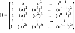
Parity check matrix for RS(n, k) code is as follows:

Let received vector be r = (r0, r1, r2, . . . , rn−1):
s= r HT = (r0, r1, r2, . . . , rn-1) 
= (r0, r1, r2, . . . , rn-1) 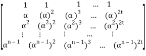
= (r0 , r0, r0, . . . , r0) + (r1α, r1(α)2, r1(α)3 , . . . , r1(α)2t)+ . . . + (rn-1 αn-1 , rn-1(αn-1)2, rn-1(αn-1)3, . . . , rn-1(αn-1)2t)
= (r0 + r1α + r2α2 + . . . + rn-1αn-1, r0+ r1(α)2+r2(α2)2 + . . . + rn-1(αn-1)2, . . . , r0 + r1(α)2t + r2(α2)2t + . . . + rn-1(αn-1)2t)
= (
= (
It can be noticed, that computing particular syndrome elements is computing value of polynomial r(x), where r(x) = rn−1x n−1 + rn−2x n−2 + . . . + r1x + r0
For RS(n, k) code, where roots of generator polynomial g(x) are consecutive 2t elements α, α2 , . . . , α2t , it is true that:
s = (r(α),r(α2 ), . . . , r(α2t ))
Particular elements of syndrome vector are:
s1 = r(α)
s2 = r(α 2 )
. . .
s2t = r(α2t)
Parity check matrix for RS(7, 3) code:

It can be written that: s = rHT = (c + e)HT = cHT + eHT = 0 + eHT = eHT
Syndrome is then dependent only from error vector, which means, that there can be created array, where syndrome vectors are assigned to error patterns. Such array has 2 columns and qn−k rows for RS(n, k) code in GF(q). Decoding is a process of computing syndrome and then finding error pattern in array which is assigned to computed syndrome. When error pattern is found, then it is added to received vector. This method is still impractical, because size of such array may be huge.
LDPC Codes
The two most important advantages of LDPC codes over turbo codes are:
- Absence of low-weight codewords and
- Iterative decoding of lower complexity.
With regard to the issue of low-weight codewords, we usually find that a small number of codewords in a turbo codeword are undesirably close to the given codeword. Owing to this closeness in weights, once in a while the channel noise causes the transmitted codeword to be mistaken for a nearby code.
In contrast, LDPC codes can be easily constructed so that they do not have such low-weight codewords and they can, therefore, achieve vanishingly small BERs. Turning next to the issue of decoding complexity, we note that the computational complexity of a turbo decoder is dominated by the MAP algorithm, which operates on the trellis for representing the convolutional code used in the encoder. The number of computations in each recursion of the MAP algorithm scales linearly with the number of states in the trellis. Commonly used turbo codes employ trellises with 16 states or more. In contrast, LDPC codes use a simple parity-check trellis that has just two states. Consequently, the decoders for LDPC codes are significantly simpler to design than those for turbo decoders. However, a practical objection to the use of LDPC codes is that, for large block lengths, their encoding complexity is high compared with turbo codes. It can be argued that LDPC codes and turbo codes complement each other, giving the designer more flexibility in selecting the right code for extraordinary decoding performance.
Construction of LDPC Codes
LDPC codes are specified by a parity-check matrix denoted by A, which is purposely chosen to be sparse; that is, the code consists mainly of 0s and a small number of 1s. In particular, we speak of (n, tc, tr) LDPC codes, where n denotes the block length, tc denotes the weight (i.e., number of 1s) in each column of the matrix A, and tr denotes the weight of each row with tr >tc. The rate of such an LDPC code is defined by
r = 1 – tc/tr
Whose validity may be justified as follows. Let denote the density of 1s in the parity check matrix A.
tc = (n – k)
tr = n
Where (n – k) is the number of rows in A and n is the number of columns (i.e., the block length). Therefore, dividing tc by tr, we get
tc/tr = 1 – k/n
The structure of LDPC codes is well portrayed by bipartite graphs, which were introduced by Tanner (1981) and, therefore, are known as Tanner graphs. Figure below shows such a graph for the example code of n = 10, tc = 3, and tr = 5. The left-hand nodes in the graph are variable (symbol) nodes, which correspond to elements of the codeword. The right-hand nodes of the graph are check nodes, which correspond to the set of parity-check constraints satisfied by codewords in the code. LDPC codes of the type exemplified by the graph of Figure below are said to be regular, in that all the nodes of a similar kind have exactly the same degree. In Figure below, the degree of the variable nodes is tc = 3 and the degree of the check nodes is tr = 5. As the block length n approaches infinity, each check node is connected to a vanishingly small fraction of variable nodes; hence the term “low density.”

Fig: Bipartite graph of the (10, 3, 5) LDPC code
The matrix A is constructed by putting 1s in A at random, subject to the regularity constraints:
- Each column of matrix A contains a small fixed number tc of 1s;
- Each row of the matrix contains a small fixed number tr of 1s.
In practice, these regularity constraints are often violated slightly in order to avoid having linearly dependent rows in the parity-check matrix A.
The parity-check matrix A of LDPC codes is not systematic (i.e., it does not have the parity-check bits appearing in diagonal form); hence the use of a symbol different from that used in Section 10.4. Nevertheless, for coding purposes, we may derive a generator matrix G for LDPC codes by means of Gaussian elimination performed in modulo-2 arithmetic. The 1-by-n code vector c is first partitioned as shown by
c = [b | m]
Where m is the k-by-1 message vector and b is the (n – k)-by-1 parity-check vector. Correspondingly, the parity-check matrix A is partitioned as
AT = [ A1 / A2]
Where A1 is a square matrix of dimensions (n – k) (n – k) and A2 is a rectangular matrix of dimensions k (n – k); transposition symbolized by the superscript T is used in the partitioning of matrix A for convenience of presentation. Imposing a constraint on the LDPC code we may write
|b|m|[A1/A2] = 0
BA1 + mA2 = 0
The vectors m and b are related by
b=mP
The coefficient matrix of LDPC codes satisfies the condition
PA1 + A2 = 0
For matrix P, we get
P =A2A1-1
The generator matrix of LDPC codes is defined by
G = [P | Ik] = [A2A1-1 | Ik]
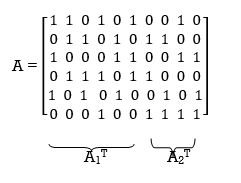
Consider the Tanner graph pertaining to a (10, 3, 5) LDPC code. The parity-check matrix of the code is defined by

Which appears to be random, while maintaining the regularity constraints: tc = 3 and tr = 5. Partitioning the matrix A in the manner just described, we write
A1 = 
A2 = 
To derive the inverse of matrix A1

Where we have introduced the vector u to denote the matrix product mA2. By using Gaussian elimination, modulo-2, the matrix A1 is transformed into lower diagonal form (i.e., all the elements above the main diagonal are zero), as shown by
A1 
This transformation is achieved by the following modulo-2 additions performed on the columns of square matrix A1:
- Columns 1 and 2 are added to column 3;
- Column 2 is added to column 4;
- Columns 1 and 4 are added to column 5;
- Columns 1, 2, and 5 are added to column 6.
Correspondingly, the vector u is transformed as shown by
u [u0, u1, u0 + u1 + u2, u1 +u3, u0 + u3 + u4, u0 + u1 + u4 + u5]
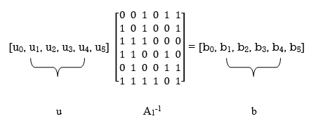
Accordingly, pre multiplying the transformed matrix A1 by the parity vector b, using successive eliminations in modulo-2 arithmetic working backwards and putting the solutions for the elements of the parity vector b in terms of the elements of the vector u in matrix form, we get

The inverse of matrix A1 is therefore
A1-1 = 
Using the given value of A2 and A1-1 the value of just found, the matrix product A2A1-1 is given by
A2A1-1 = 
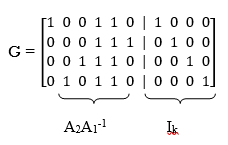
LDPC code is defined by
Key takeaway
In practice, the block length n is orders of magnitude larger than that considered in this example. Moreover, in constructing the matrix A, we may constrain all pairs of columns to have a matrix overlap (i.e., inner product of any two columns in matrix A) not to exceed one; such a constraint, over and above the regularity constraints, is expected to improve the performance of LDPC codes.
References:
1. Lathi B.P. - Modern Digital and Analog communications systems - PRISM Indian Ed.
2. Digital Communication: J.S.Chitode
3. Digital Communication (Fundamentals & applications): Bernard Scalr
4. Introduction to Error Control Codes: Salvatore Gravano
5. OFDM For wireless communication systems: Ramjee Prasad
6. Modern Communication systems (Principles and application): Leon W. Couch II (PHI)
7. Error Control Coding: Shu Lin & Daniel J.Costello
Unit - 5
Channel Coding (PART-II)
Code trellis representation
- Code trellis is the more compact representation of the code tree. In the code tree there are four states (or nodes). Every state goes to some other state depending upon the input message bit.
- Code trellis represents the single and unique diagram for such steady state transitions. The Figure below shows the code trellis diagram.
- The nodes on the left denote four possible current states and those on the right represents next state. The solid transition line represents for input message m0 = 0 and dashed line represents input message m0 = 1.
- Along with each transition line, the encoder output x1 x2 is represented during that transition.
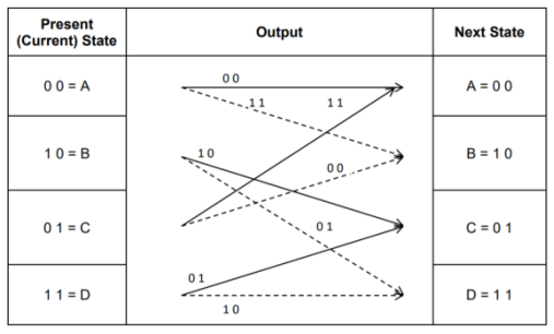
Fig: Code Trellis
Advantages of convolutional codes
- The convolutional codes operate on smaller blocks of data. Hence decoding delay is small.
- The storage hardware required is less.
Disadvantages of convolutional codes
- Due to complexity, the convolutional codes are difficult to analyze.
- These codes are not developed much as compared to block codes.
Unit - 5
Channel Coding (PART-II)
Code trellis representation
- Code trellis is the more compact representation of the code tree. In the code tree there are four states (or nodes). Every state goes to some other state depending upon the input message bit.
- Code trellis represents the single and unique diagram for such steady state transitions. The Figure below shows the code trellis diagram.
- The nodes on the left denote four possible current states and those on the right represents next state. The solid transition line represents for input message m0 = 0 and dashed line represents input message m0 = 1.
- Along with each transition line, the encoder output x1 x2 is represented during that transition.

Fig: Code Trellis
Advantages of convolutional codes
- The convolutional codes operate on smaller blocks of data. Hence decoding delay is small.
- The storage hardware required is less.
Disadvantages of convolutional codes
- Due to complexity, the convolutional codes are difficult to analyze.
- These codes are not developed much as compared to block codes.
The use of a good code with random-like properties is basic to turbo coding. In the first successful implementation of turbo codes11, Berrouet al. Achieved this design objective by using concatenated codes. The original idea of concatenated codes was conceived by Forney (1966). To be more specific, concatenated codes can be of two types: parallel or serial. The type of concatenated codes used by Berrou et al. Was of the parallel type, which is discussed in this section

Fig: Block diagram of turbo encoder of the parallel type.
Figure above depicts the most basic form of a turbo code generator that consists of two constituent systematic encoders, which are concatenated by means of an interleaver. The interleaver is an input–output mapping device that permutes the ordering of a sequence of symbols from a fixed alphabet in a completely deterministic manner; that is, it takes the symbols at the input and produces identical symbols at the output but in a different temporal order. Turbo codes use a pseudo-random interleaver, which operates only on the systematic (i.e., message) bits. The size of the interleaver used in turbo codes is typically very large, on the order of several thousand bits. There are two reasons for the use of an interleaver in a turbo code:
1. The interleaver ties together errors that are easily made in one half of the turbo code to errors that are exceptionally unlikely to occur in the other half; this is indeed one reason why the turbo code performs better than a traditional code.
2. The interleaver provides robust performance with respect to mismatched decoding, a problem that arises when the channel statistics are not known or have been incorrectly specified.
Ordinarily, but not necessarily, the same code is used for both constituent encoders in Figure above. The constituent codes recommended for turbo codes are short constraint length RSC codes. The reason for making the convolutional codes recursive (i.e., feeding one or more of the tap outputs in the shift register back to the input) is to make the internal state of the shift register depend on past outputs. This affects the behavior of the error patterns, with the result that a better performance of the overall coding strategy is attained.
Two-State Turbo Encoder Figure below shows the block diagram of a specific turbo encoder using an identical pair of two-state RSC constituent encoders. The generator matrix of each constituent encoder is given by
G(D)= (1, 1/1+D)
The input sequence of bits has length, made up of three message bits and one termination bit. The input vector is given by
m= m0 m1 m2 m3
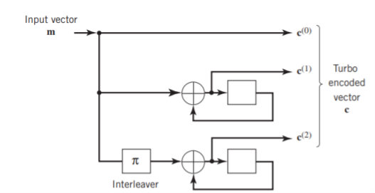
Fig: Two-state turbo encoder for Example
The parity-check vector produced by the first constituent encoder is given by
b(1) = (b0(1), b1(1), b2(1) b3(1))
Similarly, the parity-check vector produced by the second constituent encoder is given by
b(2) = (b0(2), b1(2), b2(2) b3(2))
The transmitted code vector is therefore defined by
c = (c(0), c(1), c(2))
With the convolutional code being systematic, we thus have
c(0) = m
As for the remaining two sub-vectors constituting the code vector c, they are defined by c(1) = b(1) and c(2) = b(2).
The transmitted code vector c is therefore made up of 12 bits. However, recalling that the termination bit m3 is not a message bit, it follows that the code rate of the turbo code
R=3/12=1/4
Turbo Decoder
Figure 11(a) below shows the block diagram of the two-stage turbo decoder. The decoder operates on noisy versions of the systematic bits and the two sets of parity-check bits in two decoding stages to produce an estimate of the original message bits. A distinctive feature of the turbo decoder that is immediately apparent from the block diagram of Figure11(a) is the use of feedback, manifesting itself in producing extrinsic information from one decoder to the next in an iterative manner. In a way, this decoding process is analogous to the feedback of exhaust gases experienced in a turbo-charged engine; indeed, turbo codes derive their name from this analogy. In other words, the term “turbo” in turbo codes has more to do with the decoding rather than the encoding process. In operational terms, the turbo encoder in Figure11(a) operates on noisy versions of the following inputs, obtained by demultiplexing the channel output, rj
- Systematic (i.e., message) bits, denoted by rj(0)
- Parity-check bits corresponding to encoder 1 in Figure encoder, denoted by rj(1)
- Parity-check bits corresponding to encoder 2 in Figure encoder, denoted by rj(2)
The net result of the decoding algorithm, given the received vector rj, is an estimate of the original message vector, namely, which is delivered at the decoder output to the user. Another important point to note in the turbo decoder of Figure (a) is the way in which the interleaver and de-interleaver are positioned inside the feedback loop. Bearing in mind the fact that the definition of extrinsic information requires the use of intrinsic information, we see that decoder 1 operates on three inputs:
- The noisy systematic (i.e., original message) bits,
- The noisy parity-check bits due to encoder 1, and
- De-interleaved extrinsic information computed by decoder 2

(a)

(b)
Fig: (a) Block diagram of turbo decoder. (b) Extrinsic form of turbo decoder, where I stand for interleaver, D for deinterleaver, and BCJR for BCJR for BCJR algorithm for log-MAP decoding.
In a complementary manner, decoder 2 operates on two inputs of its own:
- The noisy parity-check bits due to encoder 2 and
- The interleaved version of the extrinsic information computed by decoder 1.
- For this iterative exchange of information between the two decoders inside the feedback loop to continuously reinforce each other, the de-interleaver and interleaver would have to separate the two decoders in the manner depicted in Figure a. Moreover, the structure of the decoder in the receiver is configured to be consistent with the structure of the encoder in the transmitter.
Reed-Solomon code is error-correction code. Error-correction is such code, which can be used for error correction. Furthermore, Reed Solomon code is:
- Linear code, where result of linear combination of any two codewords is codeword,
- Cyclic code, where result of cyclic shift of codeword is codeword,
- Block code, where data sequence is divided into blocks of fixed lengths and these blocks are coded independently,
- Nonbinary code, where code symbols are not binary - 1 nor 0.
Codeword is ordered set of code symbols and belongs to code. Code symbols are elements in GF(q), which are used to code construction. Reed-Solomon, where codeword is of length n elements and encodes k information elements, is denoted as RS(n, k). Code RS(n, k) has following properties:
• codeword consists of n code symbols,
• codeword encodes k information elements,
• number of redundant control elements is r = n − k,
• code has correction capability equals to t = [r/2],
• minimal Hamming distance is dmin = r + 1.
Code can correct all error patterns, where number of errors is less or equal error capability t. Minimal Hamming distance dmin determines minimal number of positions, where two vectors are different. If code is created over GF(2m), then code is of form RS(2m− 1, 2m− 1 − 2t). Reed-Solomon codes satisfies Singleton bound with equality–dmin ≤ n − k + 1, which means, that has the best error-correction capability with given n and given information elements k. Codes which satisfy Singleton bound with equality are called MDS codes - Maximum Distance Separable.
Encoding
Encoding is process of transformation information elements into codeword. There are presented two methods for creation of Reed-Solomon codeword. Given are information elements mi ∈ GF(2m) for 0 ≤i ≤ k − 1, which are used for codeword construction.
m(x) = mk-1xk-1 + mk-2xk-2 + . . . + m1x + m0
Given is set of different non-zero elements in GF(q) which is called support set
(α1, α2, . . . , αn)
Codeword of RS(n, k) code can be expressed as:
c = (m(α1), m(α2) , . . . , m(αn))
Codeword of RS(n, k) code created with support set can be expressed as:
(1, α, α2, . . . , αn-1)
c = (m(1), m(α), . . . , m(αn-1))
c(x) = m(αn-1)xn-1 + m(αn-2)xn-2 + . . . +m(α)x + m(1)
For codeword of RS(n, k) code created with support set satisfied is that:
c(α) = c(α2) = . . . = c(α2t) = 0
Equation for Galois Field Fourier Transform for polynomial f(x) of degree n − 1 is as follows
F(x) = GFFT(f(x)) = f(1) + f(α)x + f(α2)x2 + . . . + f(αn-1)xn-1
With use of this equation, there can be shown for codeword c(x) of RS(n, k) code created with support set that 2t next coefficients are equal to zero. Codeword c(x) is in encoded in time domain, and C(x) is encoded in frequency domain.
RS code as nonbinary BCH code
Reed-Solomon codes can be seen as nonbinary BCH codes. For construction of codeword of RS(n, k) code can be used following generator polynomial:
g(x) = (x – α)(x – α2) . . . (x – α2t) where αi ∈ GF (n + 1)
Given is information polynomial m(x). Codeword of non-systematic code RS(n, k) is as follows:
c(x) = m(x)g(x)
Codeword of systematic RS(n, k) code is as follows:
c(x) = m(x)x2t + Q(x)
Q(x) = m(x)x2t mod g(x)
RS(n, k) code can be created with use of original method and as nonbinary BCH code. Both of these codes satisfy:
• code created with both definitions creates the same linear space,
• code created with both definitions is cyclic,
• for codeword created by both definitions satisfied is
c(α1) = c(α2) = . . . = c(α2t) = 0 for some 2t consecutive elements in GF(q).
Decoding algorithms
Decoding is a process of transformation of received vector from communication channel onto sequence of information elements which were used to create codeword. It may happen that received vector is not codeword, because codeword was corrupted in communication channel. In this case code can correct number of errors up to value of error correction capability. If decoder is not able to correct received vector and such situation can be recognized then it is called decoder failure. If there occurred so many errors that received vector is decoded onto different codeword than original, then such situation is called decoder error.
Complete Decoder
Complete decoder works as follows:
1. Compute Hamming distance between received vector and each codeword of RS(n, k) code,
2. Choose codeword, where value of Hamming distance was least. Complete decoder is impractical, because there are qk of codewords of RS(n, k) code and it would take much time to find result.
S
Tandard Array
Standard array is such matrix of RS(n, k) which consists of q k columns and q n−k rows. In first rows there are written all q k codewords of RS(n, k) code, and in last rows vectors which are close to them within Hamming distance. Decoding is a process of finding received vector in standard array and result of decoding is codeword in first row of the same column where received vector was found. This method is also impractical, because there must be stored q n vectors, which may be huge number.
Syndrome decoding
RS(n, k) code is a k-dimensional subspace of n-dimensional space. It is connected with two following matrices. Generator matrix G, which consists of k linear independent vectors, which are used to create codeword – c = mG, where m denotes kdimensional vector of information elements,parity check matrix H, which is used to decode received vector. Parity check matrix is used to compute syndromes. Syndrome s is computed as follows:
s = rHT,
Where r denotes received vector, and HT is transposed matrix H. If received vector is codeword, then syndrome is zero-value vector – s = cHT = 0, else there are errors, which can be written that to codeword in communication channel was added error vector – r = c + e, where e denotes error vector. For RS(n, k) code generator matrix is as follows:

Examples
Given is RS(7, 3) code created in GF(8) by polynomial p(x) = x 3 + x + 1. Generator matrix G is as follows:

For m= (α,α2,1)

=(α, α, α, α, α, α, α) + (α2, α3, α4, α5, α6, 1, α) + (1, α2, α4, α6, α, α3, α5)
= (α5, α6, α, 0, α6, 0, α5)
Construction of codeword with matrix G gives the same results as to use original method. Let m→ m(x): (α, α2, 1) →α + α2x + x2
Using original method of encoding 3.3:
c = (m(1), m(α), m(α2), m(α3 ), m(α4 ), m(α5 ), m(α6 )) = (α5 , α6 , α, 0, α6 , 0, α5 )
Parity check matrix for RS(n, k) code is as follows:
Let received vector be r = (r0, r1, r2, . . . , rn−1):
s= r HT = (r0, r1, r2, . . . , rn-1) 
= (r0, r1, r2, . . . , rn-1) 
= (r0 , r0, r0, . . . , r0) + (r1α, r1(α)2, r1(α)3 , . . . , r1(α)2t)+ . . . + (rn-1 αn-1 , rn-1(αn-1)2, rn-1(αn-1)3, . . . , rn-1(αn-1)2t)
= (r0 + r1α + r2α2 + . . . + rn-1αn-1, r0+ r1(α)2+r2(α2)2 + . . . + rn-1(αn-1)2, . . . , r0 + r1(α)2t + r2(α2)2t + . . . + rn-1(αn-1)2t)
= (
= (
It can be noticed, that computing particular syndrome elements is computing value of polynomial r(x), where r(x) = rn−1x n−1 + rn−2x n−2 + . . . + r1x + r0
For RS(n, k) code, where roots of generator polynomial g(x) are consecutive 2t elements α, α2 , . . . , α2t , it is true that:
s = (r(α),r(α2 ), . . . , r(α2t ))
Particular elements of syndrome vector are:
s1 = r(α)
s2 = r(α 2 )
. . .
s2t = r(α2t)
Parity check matrix for RS(7, 3) code:

It can be written that: s = rHT = (c + e)HT = cHT + eHT = 0 + eHT = eHT
Syndrome is then dependent only from error vector, which means, that there can be created array, where syndrome vectors are assigned to error patterns. Such array has 2 columns and qn−k rows for RS(n, k) code in GF(q). Decoding is a process of computing syndrome and then finding error pattern in array which is assigned to computed syndrome. When error pattern is found, then it is added to received vector. This method is still impractical, because size of such array may be huge.
LDPC Codes
The two most important advantages of LDPC codes over turbo codes are:
- Absence of low-weight codewords and
- Iterative decoding of lower complexity.
With regard to the issue of low-weight codewords, we usually find that a small number of codewords in a turbo codeword are undesirably close to the given codeword. Owing to this closeness in weights, once in a while the channel noise causes the transmitted codeword to be mistaken for a nearby code.
In contrast, LDPC codes can be easily constructed so that they do not have such low-weight codewords and they can, therefore, achieve vanishingly small BERs. Turning next to the issue of decoding complexity, we note that the computational complexity of a turbo decoder is dominated by the MAP algorithm, which operates on the trellis for representing the convolutional code used in the encoder. The number of computations in each recursion of the MAP algorithm scales linearly with the number of states in the trellis. Commonly used turbo codes employ trellises with 16 states or more. In contrast, LDPC codes use a simple parity-check trellis that has just two states. Consequently, the decoders for LDPC codes are significantly simpler to design than those for turbo decoders. However, a practical objection to the use of LDPC codes is that, for large block lengths, their encoding complexity is high compared with turbo codes. It can be argued that LDPC codes and turbo codes complement each other, giving the designer more flexibility in selecting the right code for extraordinary decoding performance.
Construction of LDPC Codes
LDPC codes are specified by a parity-check matrix denoted by A, which is purposely chosen to be sparse; that is, the code consists mainly of 0s and a small number of 1s. In particular, we speak of (n, tc, tr) LDPC codes, where n denotes the block length, tc denotes the weight (i.e., number of 1s) in each column of the matrix A, and tr denotes the weight of each row with tr >tc. The rate of such an LDPC code is defined by
r = 1 – tc/tr
Whose validity may be justified as follows. Let denote the density of 1s in the parity check matrix A.
tc = (n – k)
tr = n
Where (n – k) is the number of rows in A and n is the number of columns (i.e., the block length). Therefore, dividing tc by tr, we get
tc/tr = 1 – k/n
The structure of LDPC codes is well portrayed by bipartite graphs, which were introduced by Tanner (1981) and, therefore, are known as Tanner graphs. Figure below shows such a graph for the example code of n = 10, tc = 3, and tr = 5. The left-hand nodes in the graph are variable (symbol) nodes, which correspond to elements of the codeword. The right-hand nodes of the graph are check nodes, which correspond to the set of parity-check constraints satisfied by codewords in the code. LDPC codes of the type exemplified by the graph of Figure below are said to be regular, in that all the nodes of a similar kind have exactly the same degree. In Figure below, the degree of the variable nodes is tc = 3 and the degree of the check nodes is tr = 5. As the block length n approaches infinity, each check node is connected to a vanishingly small fraction of variable nodes; hence the term “low density.”

Fig: Bipartite graph of the (10, 3, 5) LDPC code
The matrix A is constructed by putting 1s in A at random, subject to the regularity constraints:
- Each column of matrix A contains a small fixed number tc of 1s;
- Each row of the matrix contains a small fixed number tr of 1s.
In practice, these regularity constraints are often violated slightly in order to avoid having linearly dependent rows in the parity-check matrix A.
The parity-check matrix A of LDPC codes is not systematic (i.e., it does not have the parity-check bits appearing in diagonal form); hence the use of a symbol different from that used in Section 10.4. Nevertheless, for coding purposes, we may derive a generator matrix G for LDPC codes by means of Gaussian elimination performed in modulo-2 arithmetic. The 1-by-n code vector c is first partitioned as shown by
c = [b | m]
Where m is the k-by-1 message vector and b is the (n – k)-by-1 parity-check vector. Correspondingly, the parity-check matrix A is partitioned as
AT = [ A1 / A2]
Where A1 is a square matrix of dimensions (n – k) (n – k) and A2 is a rectangular matrix of dimensions k (n – k); transposition symbolized by the superscript T is used in the partitioning of matrix A for convenience of presentation. Imposing a constraint on the LDPC code we may write
|b|m|[A1/A2] = 0
BA1 + mA2 = 0
The vectors m and b are related by
b=mP
The coefficient matrix of LDPC codes satisfies the condition
PA1 + A2 = 0
For matrix P, we get
P =A2A1-1
The generator matrix of LDPC codes is defined by
G = [P | Ik] = [A2A1-1 | Ik]
Consider the Tanner graph pertaining to a (10, 3, 5) LDPC code. The parity-check matrix of the code is defined by

Which appears to be random, while maintaining the regularity constraints: tc = 3 and tr = 5. Partitioning the matrix A in the manner just described, we write
A1 = 
A2 = 
To derive the inverse of matrix A1

Where we have introduced the vector u to denote the matrix product mA2. By using Gaussian elimination, modulo-2, the matrix A1 is transformed into lower diagonal form (i.e., all the elements above the main diagonal are zero), as shown by
A1 
This transformation is achieved by the following modulo-2 additions performed on the columns of square matrix A1:
- Columns 1 and 2 are added to column 3;
- Column 2 is added to column 4;
- Columns 1 and 4 are added to column 5;
- Columns 1, 2, and 5 are added to column 6.
Correspondingly, the vector u is transformed as shown by
u [u0, u1, u0 + u1 + u2, u1 +u3, u0 + u3 + u4, u0 + u1 + u4 + u5]
Accordingly, pre multiplying the transformed matrix A1 by the parity vector b, using successive eliminations in modulo-2 arithmetic working backwards and putting the solutions for the elements of the parity vector b in terms of the elements of the vector u in matrix form, we get
The inverse of matrix A1 is therefore
A1-1 = 
Using the given value of A2 and A1-1 the value of just found, the matrix product A2A1-1 is given by
A2A1-1 = 
LDPC code is defined by

Key takeaway
In practice, the block length n is orders of magnitude larger than that considered in this example. Moreover, in constructing the matrix A, we may constrain all pairs of columns to have a matrix overlap (i.e., inner product of any two columns in matrix A) not to exceed one; such a constraint, over and above the regularity constraints, is expected to improve the performance of LDPC codes.
References:
1. Lathi B.P. - Modern Digital and Analog communications systems - PRISM Indian Ed.
2. Digital Communication: J.S.Chitode
3. Digital Communication (Fundamentals & applications): Bernard Scalr
4. Introduction to Error Control Codes: Salvatore Gravano
5. OFDM For wireless communication systems: Ramjee Prasad
6. Modern Communication systems (Principles and application): Leon W. Couch II (PHI)
7. Error Control Coding: Shu Lin & Daniel J.Costello
Unit - 5
Channel Coding (PART-II)
Code trellis representation
- Code trellis is the more compact representation of the code tree. In the code tree there are four states (or nodes). Every state goes to some other state depending upon the input message bit.
- Code trellis represents the single and unique diagram for such steady state transitions. The Figure below shows the code trellis diagram.
- The nodes on the left denote four possible current states and those on the right represents next state. The solid transition line represents for input message m0 = 0 and dashed line represents input message m0 = 1.
- Along with each transition line, the encoder output x1 x2 is represented during that transition.

Fig: Code Trellis
Advantages of convolutional codes
- The convolutional codes operate on smaller blocks of data. Hence decoding delay is small.
- The storage hardware required is less.
Disadvantages of convolutional codes
- Due to complexity, the convolutional codes are difficult to analyze.
- These codes are not developed much as compared to block codes.
The use of a good code with random-like properties is basic to turbo coding. In the first successful implementation of turbo codes11, Berrouet al. Achieved this design objective by using concatenated codes. The original idea of concatenated codes was conceived by Forney (1966). To be more specific, concatenated codes can be of two types: parallel or serial. The type of concatenated codes used by Berrou et al. Was of the parallel type, which is discussed in this section
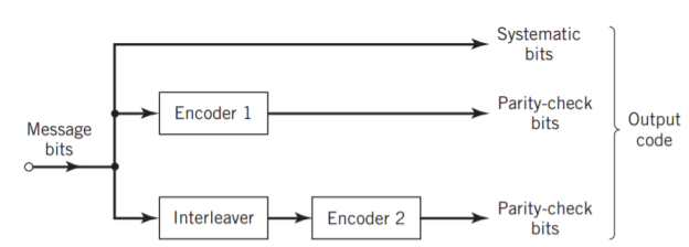
Fig: Block diagram of turbo encoder of the parallel type.
Figure above depicts the most basic form of a turbo code generator that consists of two constituent systematic encoders, which are concatenated by means of an interleaver. The interleaver is an input–output mapping device that permutes the ordering of a sequence of symbols from a fixed alphabet in a completely deterministic manner; that is, it takes the symbols at the input and produces identical symbols at the output but in a different temporal order. Turbo codes use a pseudo-random interleaver, which operates only on the systematic (i.e., message) bits. The size of the interleaver used in turbo codes is typically very large, on the order of several thousand bits. There are two reasons for the use of an interleaver in a turbo code:
1. The interleaver ties together errors that are easily made in one half of the turbo code to errors that are exceptionally unlikely to occur in the other half; this is indeed one reason why the turbo code performs better than a traditional code.
2. The interleaver provides robust performance with respect to mismatched decoding, a problem that arises when the channel statistics are not known or have been incorrectly specified.
Ordinarily, but not necessarily, the same code is used for both constituent encoders in Figure above. The constituent codes recommended for turbo codes are short constraint length RSC codes. The reason for making the convolutional codes recursive (i.e., feeding one or more of the tap outputs in the shift register back to the input) is to make the internal state of the shift register depend on past outputs. This affects the behavior of the error patterns, with the result that a better performance of the overall coding strategy is attained.
Two-State Turbo Encoder Figure below shows the block diagram of a specific turbo encoder using an identical pair of two-state RSC constituent encoders. The generator matrix of each constituent encoder is given by
G(D)= (1, 1/1+D)
The input sequence of bits has length, made up of three message bits and one termination bit. The input vector is given by
m= m0 m1 m2 m3

Fig: Two-state turbo encoder for Example
The parity-check vector produced by the first constituent encoder is given by
b(1) = (b0(1), b1(1), b2(1) b3(1))
Similarly, the parity-check vector produced by the second constituent encoder is given by
b(2) = (b0(2), b1(2), b2(2) b3(2))
The transmitted code vector is therefore defined by
c = (c(0), c(1), c(2))
With the convolutional code being systematic, we thus have
c(0) = m
As for the remaining two sub-vectors constituting the code vector c, they are defined by c(1) = b(1) and c(2) = b(2).
The transmitted code vector c is therefore made up of 12 bits. However, recalling that the termination bit m3 is not a message bit, it follows that the code rate of the turbo code
R=3/12=1/4
Turbo Decoder
Figure 11(a) below shows the block diagram of the two-stage turbo decoder. The decoder operates on noisy versions of the systematic bits and the two sets of parity-check bits in two decoding stages to produce an estimate of the original message bits. A distinctive feature of the turbo decoder that is immediately apparent from the block diagram of Figure11(a) is the use of feedback, manifesting itself in producing extrinsic information from one decoder to the next in an iterative manner. In a way, this decoding process is analogous to the feedback of exhaust gases experienced in a turbo-charged engine; indeed, turbo codes derive their name from this analogy. In other words, the term “turbo” in turbo codes has more to do with the decoding rather than the encoding process. In operational terms, the turbo encoder in Figure11(a) operates on noisy versions of the following inputs, obtained by demultiplexing the channel output, rj
- Systematic (i.e., message) bits, denoted by rj(0)
- Parity-check bits corresponding to encoder 1 in Figure encoder, denoted by rj(1)
- Parity-check bits corresponding to encoder 2 in Figure encoder, denoted by rj(2)
The net result of the decoding algorithm, given the received vector rj, is an estimate of the original message vector, namely, which is delivered at the decoder output to the user. Another important point to note in the turbo decoder of Figure (a) is the way in which the interleaver and de-interleaver are positioned inside the feedback loop. Bearing in mind the fact that the definition of extrinsic information requires the use of intrinsic information, we see that decoder 1 operates on three inputs:
- The noisy systematic (i.e., original message) bits,
- The noisy parity-check bits due to encoder 1, and
- De-interleaved extrinsic information computed by decoder 2

(a)

(b)
Fig: (a) Block diagram of turbo decoder. (b) Extrinsic form of turbo decoder, where I stand for interleaver, D for deinterleaver, and BCJR for BCJR for BCJR algorithm for log-MAP decoding.
In a complementary manner, decoder 2 operates on two inputs of its own:
- The noisy parity-check bits due to encoder 2 and
- The interleaved version of the extrinsic information computed by decoder 1.
- For this iterative exchange of information between the two decoders inside the feedback loop to continuously reinforce each other, the de-interleaver and interleaver would have to separate the two decoders in the manner depicted in Figure a. Moreover, the structure of the decoder in the receiver is configured to be consistent with the structure of the encoder in the transmitter.
Reed-Solomon code is error-correction code. Error-correction is such code, which can be used for error correction. Furthermore, Reed Solomon code is:
- Linear code, where result of linear combination of any two codewords is codeword,
- Cyclic code, where result of cyclic shift of codeword is codeword,
- Block code, where data sequence is divided into blocks of fixed lengths and these blocks are coded independently,
- Nonbinary code, where code symbols are not binary - 1 nor 0.
Codeword is ordered set of code symbols and belongs to code. Code symbols are elements in GF(q), which are used to code construction. Reed-Solomon, where codeword is of length n elements and encodes k information elements, is denoted as RS(n, k). Code RS(n, k) has following properties:
• codeword consists of n code symbols,
• codeword encodes k information elements,
• number of redundant control elements is r = n − k,
• code has correction capability equals to t = [r/2],
• minimal Hamming distance is dmin = r + 1.
Code can correct all error patterns, where number of errors is less or equal error capability t. Minimal Hamming distance dmin determines minimal number of positions, where two vectors are different. If code is created over GF(2m), then code is of form RS(2m− 1, 2m− 1 − 2t). Reed-Solomon codes satisfies Singleton bound with equality–dmin ≤ n − k + 1, which means, that has the best error-correction capability with given n and given information elements k. Codes which satisfy Singleton bound with equality are called MDS codes - Maximum Distance Separable.
Encoding
Encoding is process of transformation information elements into codeword. There are presented two methods for creation of Reed-Solomon codeword. Given are information elements mi ∈ GF(2m) for 0 ≤i ≤ k − 1, which are used for codeword construction.
m(x) = mk-1xk-1 + mk-2xk-2 + . . . + m1x + m0
Given is set of different non-zero elements in GF(q) which is called support set
(α1, α2, . . . , αn)
Codeword of RS(n, k) code can be expressed as:
c = (m(α1), m(α2) , . . . , m(αn))
Codeword of RS(n, k) code created with support set can be expressed as:
(1, α, α2, . . . , αn-1)
c = (m(1), m(α), . . . , m(αn-1))
c(x) = m(αn-1)xn-1 + m(αn-2)xn-2 + . . . +m(α)x + m(1)
For codeword of RS(n, k) code created with support set satisfied is that:
c(α) = c(α2) = . . . = c(α2t) = 0
Equation for Galois Field Fourier Transform for polynomial f(x) of degree n − 1 is as follows
F(x) = GFFT(f(x)) = f(1) + f(α)x + f(α2)x2 + . . . + f(αn-1)xn-1
With use of this equation, there can be shown for codeword c(x) of RS(n, k) code created with support set that 2t next coefficients are equal to zero. Codeword c(x) is in encoded in time domain, and C(x) is encoded in frequency domain.
RS code as nonbinary BCH code
Reed-Solomon codes can be seen as nonbinary BCH codes. For construction of codeword of RS(n, k) code can be used following generator polynomial:
g(x) = (x – α)(x – α2) . . . (x – α2t) where αi ∈ GF (n + 1)
Given is information polynomial m(x). Codeword of non-systematic code RS(n, k) is as follows:
c(x) = m(x)g(x)
Codeword of systematic RS(n, k) code is as follows:
c(x) = m(x)x2t + Q(x)
Q(x) = m(x)x2t mod g(x)
RS(n, k) code can be created with use of original method and as nonbinary BCH code. Both of these codes satisfy:
• code created with both definitions creates the same linear space,
• code created with both definitions is cyclic,
• for codeword created by both definitions satisfied is
c(α1) = c(α2) = . . . = c(α2t) = 0 for some 2t consecutive elements in GF(q).
Decoding algorithms
Decoding is a process of transformation of received vector from communication channel onto sequence of information elements which were used to create codeword. It may happen that received vector is not codeword, because codeword was corrupted in communication channel. In this case code can correct number of errors up to value of error correction capability. If decoder is not able to correct received vector and such situation can be recognized then it is called decoder failure. If there occurred so many errors that received vector is decoded onto different codeword than original, then such situation is called decoder error.
Complete Decoder
Complete decoder works as follows:
1. Compute Hamming distance between received vector and each codeword of RS(n, k) code,
2. Choose codeword, where value of Hamming distance was least. Complete decoder is impractical, because there are qk of codewords of RS(n, k) code and it would take much time to find result.
S
Tandard Array
Standard array is such matrix of RS(n, k) which consists of q k columns and q n−k rows. In first rows there are written all q k codewords of RS(n, k) code, and in last rows vectors which are close to them within Hamming distance. Decoding is a process of finding received vector in standard array and result of decoding is codeword in first row of the same column where received vector was found. This method is also impractical, because there must be stored q n vectors, which may be huge number.
Syndrome decoding
RS(n, k) code is a k-dimensional subspace of n-dimensional space. It is connected with two following matrices. Generator matrix G, which consists of k linear independent vectors, which are used to create codeword – c = mG, where m denotes kdimensional vector of information elements,parity check matrix H, which is used to decode received vector. Parity check matrix is used to compute syndromes. Syndrome s is computed as follows:
s = rHT,
Where r denotes received vector, and HT is transposed matrix H. If received vector is codeword, then syndrome is zero-value vector – s = cHT = 0, else there are errors, which can be written that to codeword in communication channel was added error vector – r = c + e, where e denotes error vector. For RS(n, k) code generator matrix is as follows:

Examples
Given is RS(7, 3) code created in GF(8) by polynomial p(x) = x 3 + x + 1. Generator matrix G is as follows:

For m= (α,α2,1)

=(α, α, α, α, α, α, α) + (α2, α3, α4, α5, α6, 1, α) + (1, α2, α4, α6, α, α3, α5)
= (α5, α6, α, 0, α6, 0, α5)
Construction of codeword with matrix G gives the same results as to use original method. Let m→ m(x): (α, α2, 1) →α + α2x + x2
Using original method of encoding 3.3:
c = (m(1), m(α), m(α2), m(α3 ), m(α4 ), m(α5 ), m(α6 )) = (α5 , α6 , α, 0, α6 , 0, α5 )
Parity check matrix for RS(n, k) code is as follows:

Let received vector be r = (r0, r1, r2, . . . , rn−1):
s= r HT = (r0, r1, r2, . . . , rn-1) 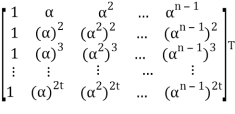
= (r0, r1, r2, . . . , rn-1) 
= (r0 , r0, r0, . . . , r0) + (r1α, r1(α)2, r1(α)3 , . . . , r1(α)2t)+ . . . + (rn-1 αn-1 , rn-1(αn-1)2, rn-1(αn-1)3, . . . , rn-1(αn-1)2t)
= (r0 + r1α + r2α2 + . . . + rn-1αn-1, r0+ r1(α)2+r2(α2)2 + . . . + rn-1(αn-1)2, . . . , r0 + r1(α)2t + r2(α2)2t + . . . + rn-1(αn-1)2t)
= (
= (
It can be noticed, that computing particular syndrome elements is computing value of polynomial r(x), where r(x) = rn−1x n−1 + rn−2x n−2 + . . . + r1x + r0
For RS(n, k) code, where roots of generator polynomial g(x) are consecutive 2t elements α, α2 , . . . , α2t , it is true that:
s = (r(α),r(α2 ), . . . , r(α2t ))
Particular elements of syndrome vector are:
s1 = r(α)
s2 = r(α 2 )
. . .
s2t = r(α2t)
Parity check matrix for RS(7, 3) code:

It can be written that: s = rHT = (c + e)HT = cHT + eHT = 0 + eHT = eHT
Syndrome is then dependent only from error vector, which means, that there can be created array, where syndrome vectors are assigned to error patterns. Such array has 2 columns and qn−k rows for RS(n, k) code in GF(q). Decoding is a process of computing syndrome and then finding error pattern in array which is assigned to computed syndrome. When error pattern is found, then it is added to received vector. This method is still impractical, because size of such array may be huge.
LDPC Codes
The two most important advantages of LDPC codes over turbo codes are:
- Absence of low-weight codewords and
- Iterative decoding of lower complexity.
With regard to the issue of low-weight codewords, we usually find that a small number of codewords in a turbo codeword are undesirably close to the given codeword. Owing to this closeness in weights, once in a while the channel noise causes the transmitted codeword to be mistaken for a nearby code.
In contrast, LDPC codes can be easily constructed so that they do not have such low-weight codewords and they can, therefore, achieve vanishingly small BERs. Turning next to the issue of decoding complexity, we note that the computational complexity of a turbo decoder is dominated by the MAP algorithm, which operates on the trellis for representing the convolutional code used in the encoder. The number of computations in each recursion of the MAP algorithm scales linearly with the number of states in the trellis. Commonly used turbo codes employ trellises with 16 states or more. In contrast, LDPC codes use a simple parity-check trellis that has just two states. Consequently, the decoders for LDPC codes are significantly simpler to design than those for turbo decoders. However, a practical objection to the use of LDPC codes is that, for large block lengths, their encoding complexity is high compared with turbo codes. It can be argued that LDPC codes and turbo codes complement each other, giving the designer more flexibility in selecting the right code for extraordinary decoding performance.
Construction of LDPC Codes
LDPC codes are specified by a parity-check matrix denoted by A, which is purposely chosen to be sparse; that is, the code consists mainly of 0s and a small number of 1s. In particular, we speak of (n, tc, tr) LDPC codes, where n denotes the block length, tc denotes the weight (i.e., number of 1s) in each column of the matrix A, and tr denotes the weight of each row with tr >tc. The rate of such an LDPC code is defined by
r = 1 – tc/tr
Whose validity may be justified as follows. Let denote the density of 1s in the parity check matrix A.
tc = (n – k)
tr = n
Where (n – k) is the number of rows in A and n is the number of columns (i.e., the block length). Therefore, dividing tc by tr, we get
tc/tr = 1 – k/n
The structure of LDPC codes is well portrayed by bipartite graphs, which were introduced by Tanner (1981) and, therefore, are known as Tanner graphs. Figure below shows such a graph for the example code of n = 10, tc = 3, and tr = 5. The left-hand nodes in the graph are variable (symbol) nodes, which correspond to elements of the codeword. The right-hand nodes of the graph are check nodes, which correspond to the set of parity-check constraints satisfied by codewords in the code. LDPC codes of the type exemplified by the graph of Figure below are said to be regular, in that all the nodes of a similar kind have exactly the same degree. In Figure below, the degree of the variable nodes is tc = 3 and the degree of the check nodes is tr = 5. As the block length n approaches infinity, each check node is connected to a vanishingly small fraction of variable nodes; hence the term “low density.”
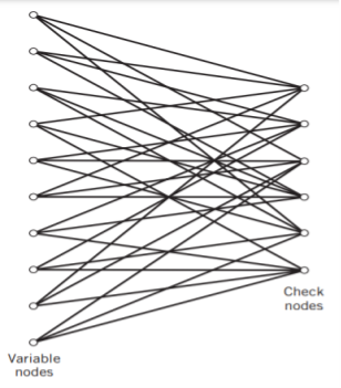
Fig: Bipartite graph of the (10, 3, 5) LDPC code
The matrix A is constructed by putting 1s in A at random, subject to the regularity constraints:
- Each column of matrix A contains a small fixed number tc of 1s;
- Each row of the matrix contains a small fixed number tr of 1s.
In practice, these regularity constraints are often violated slightly in order to avoid having linearly dependent rows in the parity-check matrix A.
The parity-check matrix A of LDPC codes is not systematic (i.e., it does not have the parity-check bits appearing in diagonal form); hence the use of a symbol different from that used in Section 10.4. Nevertheless, for coding purposes, we may derive a generator matrix G for LDPC codes by means of Gaussian elimination performed in modulo-2 arithmetic. The 1-by-n code vector c is first partitioned as shown by
c = [b | m]
Where m is the k-by-1 message vector and b is the (n – k)-by-1 parity-check vector. Correspondingly, the parity-check matrix A is partitioned as
AT = [ A1 / A2]
Where A1 is a square matrix of dimensions (n – k) (n – k) and A2 is a rectangular matrix of dimensions k (n – k); transposition symbolized by the superscript T is used in the partitioning of matrix A for convenience of presentation. Imposing a constraint on the LDPC code we may write
|b|m|[A1/A2] = 0
BA1 + mA2 = 0
The vectors m and b are related by
b=mP
The coefficient matrix of LDPC codes satisfies the condition
PA1 + A2 = 0
For matrix P, we get
P =A2A1-1
The generator matrix of LDPC codes is defined by
G = [P | Ik] = [A2A1-1 | Ik]
Consider the Tanner graph pertaining to a (10, 3, 5) LDPC code. The parity-check matrix of the code is defined by
Which appears to be random, while maintaining the regularity constraints: tc = 3 and tr = 5. Partitioning the matrix A in the manner just described, we write
A1 = 
A2 = 
To derive the inverse of matrix A1
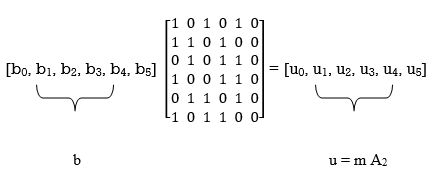
Where we have introduced the vector u to denote the matrix product mA2. By using Gaussian elimination, modulo-2, the matrix A1 is transformed into lower diagonal form (i.e., all the elements above the main diagonal are zero), as shown by
A1 
This transformation is achieved by the following modulo-2 additions performed on the columns of square matrix A1:
- Columns 1 and 2 are added to column 3;
- Column 2 is added to column 4;
- Columns 1 and 4 are added to column 5;
- Columns 1, 2, and 5 are added to column 6.
Correspondingly, the vector u is transformed as shown by
u [u0, u1, u0 + u1 + u2, u1 +u3, u0 + u3 + u4, u0 + u1 + u4 + u5]
Accordingly, pre multiplying the transformed matrix A1 by the parity vector b, using successive eliminations in modulo-2 arithmetic working backwards and putting the solutions for the elements of the parity vector b in terms of the elements of the vector u in matrix form, we get

The inverse of matrix A1 is therefore
A1-1 = 
Using the given value of A2 and A1-1 the value of just found, the matrix product A2A1-1 is given by
A2A1-1 = 
LDPC code is defined by

Key takeaway
In practice, the block length n is orders of magnitude larger than that considered in this example. Moreover, in constructing the matrix A, we may constrain all pairs of columns to have a matrix overlap (i.e., inner product of any two columns in matrix A) not to exceed one; such a constraint, over and above the regularity constraints, is expected to improve the performance of LDPC codes.
References:
1. Lathi B.P. - Modern Digital and Analog communications systems - PRISM Indian Ed.
2. Digital Communication: J.S.Chitode
3. Digital Communication (Fundamentals & applications): Bernard Scalr
4. Introduction to Error Control Codes: Salvatore Gravano
5. OFDM For wireless communication systems: Ramjee Prasad
6. Modern Communication systems (Principles and application): Leon W. Couch II (PHI)
7. Error Control Coding: Shu Lin & Daniel J.Costello