Unit - 3
Flow through Pipes
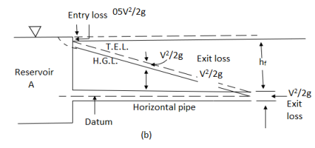
The concept of hydraulic gradient line and total energy line is quite useful in the study of flow of fluid in pipes.
Total energy Line (T.E.L. Or E.G.L)
- It is known that the total head with respect to any arbitrary datums, is the sum of the elevation (potential) head, pressure head and velocity head.
- Total head =

- When the fluid flows along the pipe, there is loss of head and the total energy decreases in the direction of flow. If the total energy at various point along the axis of the pipe is plotted and joined by a line, the line so obtained is called the Energy gradient line (E.G.L)
- Energy gradient line (E.G.L) is also known as Total energy line (T.E.L)
Hydraulic gradient Line (H.G.L)
- The sum of potential head and the pressure head

- At any point is called the piezometric head.
- If a line is drawn joining the piezometric levels at various points, the line so obtained is called the ‘Hydraulic gradient line.
- Hydraulic gradient line (H.G.L) is always below the energy gradient line (E.G.L) and the vertical intercept between the two is equal to the velocity head

Key Takeaways:
- The concept of hydraulic gradient line and total energy line is quite useful in the study of flow of fluid in pipes.
- If the total energy at various point along the axis of the pipe is plotted and joined by a line, the line so obtained is called the Energy gradient line (E.G.L)
- If a line is drawn joining the piezometric levels at various points, the line so obtained is called the ‘Hydraulic gradient line.
When water flows in a pipe, it experiences some resistance to its motion, due to which its velocity and ultimately the head of water available is reduced.
Major energy losses
This loss is due to friction.
Darcy – Weisbach formula
The loss of head in pipes due to friction is calculated from Darcy-Weisbach formula which is given by
hf = 
Where, hf = loss of head due to friction,
f = co-efficient of friction,(a function of Reynolds number, Re)
f =  for Re varying from 4000 to 106
=  for Re < 2000 (laminar/ viscous flow)
L = Lengthof the pipe
V = Mean velocity of flow, and
D = Diameter of the pipe.
Minor Energy Loses
- The loss of energy due to change of velocity of the flowing fluid in magnitude or direction is called minor loss of energy.
- The minor loss of energy (or head) includes the following cases:
Loss of head due to Sudden Enlargement.
- Consider a liquid flowing through a pipe that has sudden enlargement as shown in fig.
he = 
- Loss of head due to Sudden Contraction
- Consider a liquid flowing in a pipe that has a Sudden Contraction in the area as shown in fig.
hc = V22/ 2g [ 1/c -1]2
- Loss of head at the entrance of a pipe:
- This is the loss of energy which occurs when a liquid enters a pipe that is connected to a large tank or reservoir.
hi = 0.5 V2/2g
- Loss of head at the exit of pipe:
- This is the loss of head due to the velocity of the liquid at the outlet of the pipe which is dissipated either in the form of a free jet or it is lost in the tank or reservoir.
h0 = V2/2g
- Loss of head due to an obstruction in a pipe:
- Whenever there is an obstruction in a pipe, the loss of energy takes place due to the reduction of the area of the cross-section of the pipe at the place where the obstruction is present.
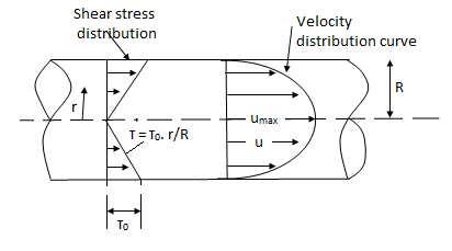
Let τ0 = Shearing stress at the pipe wall
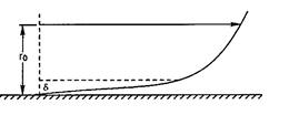
τ0 = μ× velocity gradient at the pipe wall
= μ 
At y = δ let u = uδ
∴ 
∴τ0 =μ 
∴τ0/ρ =

∴v*2 = 

a = Maximum area of obstruction
A = Area of pipe
V = Velocity of liquid in the pipe
habs = V2/2g [ A/Cc(A-a) – 1]2
- Loss of head due to bend in pipe:
- When there is any bend in a pipe, the velocity of the flow changes, due to which the separation of the flow from the boundary and also the formation of eddies takes place.
hb = kV2/2g
Where k is coefficient of bend
Loss of head in various pipe fittings:
- The loss of head in various pipe fittings such as valves, couplings, etc. is expressed as
hpf = kV2/2g
Where k is coefficient of pipe fitting
Key Takeaways:
- When water flows in a pipe, it experiences some resistance to its motion, due to which its velocity and ultimately the head of water available is reduced.
- The loss of energy due to change of velocity of the flowing fluid in magnitude or direction is called minor loss of energy.
Fig shows a horizontal pipe having steady flow.
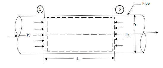
Fig: Darcy wiesbatch equation
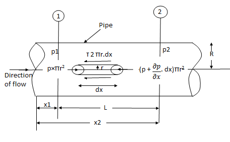
Consider control volume enclosed between section 1 and 2 of the pipe.
p1 = Intensity of pressure at section 1,
p2 = Intensity of pressure at section 2,
L = Length of the pipe, between section 1 and 2,
D = Diameter of the pipe,
f = Non-dimensional factor (Whose value depends on the material and nature of the pipe surface), and
hf= Loss of head due to friction.
Propelling force on the following fluid between the two section is = (p1 – p2) A
(Where, A = area of cross section of the pipe
Frictional resistance force = f ’ PLV
Where P = wetted perimeter, and
V = Average flow velocity
Under Equilibrium condition,
Propelling force = Frictional resistance force
i.e. (p1 – p2) A = f PLV2.
Dividing both sides by weight density W, we have
(P1 – P2/W) A = 
hf = = 
hf = 
= 
The ratio  is called the hydraulic mean depth or hydraulic radius, denoted by m (or R).
The term ( ) has dimensions of hf and thus the term
  is a non-dimensional quantity and let us replace it by another constant f.
hf = f ------- 1
In case of a circular pipe,
Hydraulic mean depth, m = 
Substituting this value in equation 1, we get
hf = f ---------2
(The factor f is known as Darcy coefficient of friction.)
Equation 2 is known as Darcy-Weisbach equation.
Key takeaways
Darcy weisbach equation
hf = f
Major loss of energy refers to the loss of head or energy caused by friction in a pipe, whereas minor loss of energy refers to the loss of energy caused by a change in magnitude or direction in the velocity of the following fluid.
- Loss of head due to sudden enlargement
- Loss of head due to sudden contraction
- Loss of head at the entrance of a pipe
- Loss of head at the exit of a pipe
- Loss of head due to an obstruction in a pipe
- Loss of head due to bend in the pipe
- Loss of head in various pipe fittings
Because the above losses are minor in comparison to the loss of head due to friction in a lengthy pipe, they are referred to as minor losses and can even be overlooked without causing major inaccuracy. In the event of a short pipe, however, these losses are comparable to head loss due to friction.
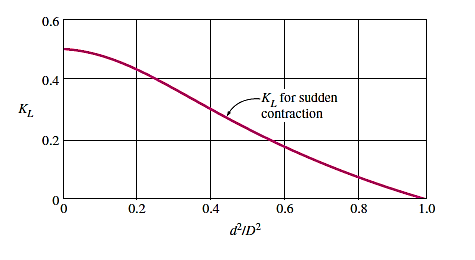
Loss of Head Due to Sudden Enlargement:
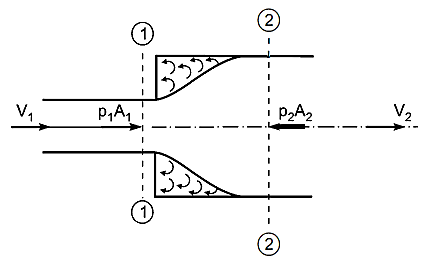
Consider a liquid flowing through a conduit that suddenly expands, as depicted. Before and after the enlargement, consider two parts (1)-(1) and (2)-(2).
Applying Bernoulli’s Equation:


he = 
Consider the control volume of liquid between sections 1-1 and 2-2. Then the force acting on the liquid in the control volume in the direction of flow is given by
Fx = p1A1 + P(A2 – A1) – p2A2
Experimentally, P = p1
Fx = p1A1 + p1(A2 – A1) – p2A2
Fx = p1A1 – p2A2
Fx = (p1 – p2) A2
Momentum of liquid/sec at section 1 – 1 = mass * velocity
= ρA1V12
Momentum of liquid/sec at section 2 – 2 = mass * velocity
= ρA2V22
Change of momentum
ρA2V22 - ρA1V12
Using continuity equation
A1V1 = A2 V2
A1 = 
Change of momentum,
ρA2V22 - ρ
Now net force acting on the control volume in the direction of flow must be equal to the rate of change of momentum or change of momentum per second.
(p1 – p2)A2 = ρA2(
(p1 – p2)/ρ = 
(p1 – p2)/ρg =  /g
/g
p1 /ρg – p2/ρg =  /g
/g
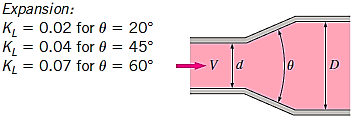
So,
he = 
he = 
he = 
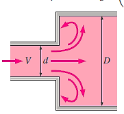
Loss of Head Due to Sudden Contraction:
Consider a liquid running through a pipe with an abrupt area contraction, as depicted. Before and after contraction, consider parts 1-1 and 2-2. As liquid flows from a large pipe to a smaller pipe, the flow area decreases until it reaches a minimum at section C-C, as depicted. Vena-contracta is the name given to this section C-C. A dramatic increase of the region occurs after section C-C. The sudden loss of head is actually owing to a sudden expansion of the Vena-contracta into a smaller channel.
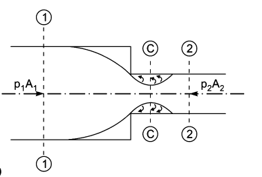
Actual loss of head due to enlargement from section C-C to section 2-2 and is given by equation,
hc =  =
= 
Using continuity equation
Ac = A2 V2/ Vc

So,
hc = 
hc = 
Where,
k = 

If,
Cc = 0.62 then k = 0.375
Then,
hc = 0.375 
If the value of Cc is not given, then the head loss due to contraction is taken as,
hc = 0.5 
Loss of Head at the Entrance of a Pipe:
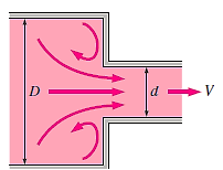
When a liquid enters a conduit that is connected to a huge tank or reservoir, there is a loss of energy. This is analogous to the loss of a head as a result of a rapid constriction. The amount of loss is determined by the type of entrance. This loss is significantly more for a sharp edge entrance than for a rounded or bell mouthed opening. The value of head loss at the entrance (or inlet) of a pipe with sharp cornered entrance is taken in practise as,
hi = 0.5 
Loss of Head at the Exit of Pipe:
This is the loss of head (or energy) caused by the velocity of liquid at the pipe's outlet, which is dissipated either as a free jet (if the pipe's outlet is free) or in the tank or reservoir (if the pipe's outlet is connected to the tank or reservoir).
ho = 0.5 
Loss of Head Due to an Obstruction in a Pipe:
When there is an impediment in a pipe, energy is lost due to a reduction in the area of the pipe's cross-section at the blockage. There is a dramatic increase of the flow region beyond the obstacle, resulting in loss of head.
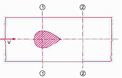
a = Maximum area of obstruction
A = Area of pipe
V = velocity of liquid in pipe
(A-a) = Area of flow of liquid at section 1 - 1
A vena-contracta is produced beyond section 1-1 as the liquid flows, after which the stream of liquid widens again and the velocity of flow at section 2-2 becomes uniform and equal to the pipe's velocity, Vin. The flow of liquid through sudden expansion is analogous to this condition.
Vc = Velocity of liquid at venacontracta
Then loss of head due to obstruction = loss of head due to enlargement from vena-contracta to section 2-2,
= (Vc – V)2/ 2g
From continuity,
ac = AV/ Vc
Then,
Cc = 
ac = Cc * (A – a)
So,
Cc × (A – a) × Vc = A × V
Vc = 
Hence,
(Vc – V)2/ 2g =  =
= 
Loss of Head due to Bend in Pipe:
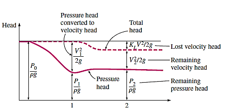
When there is a bend c in a pipe, the velocity of the flow varies, causing the flow to separate from the boundary and the development of eddies. As a result, the energy is lost. The head loss in a pipe due to bending is given as,
hb = 
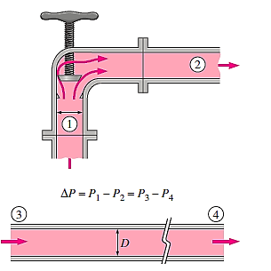
∆P = P1 – P2 = P3 – P4
The value of K depends on,
- Angle of bend
- Radius of curvature of bend
- Diameter of pipe
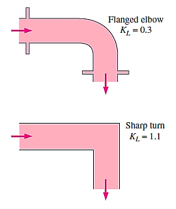
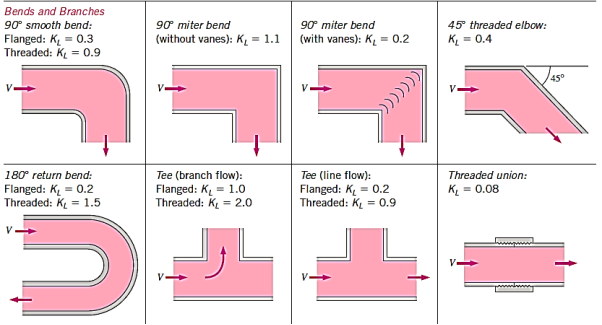
Loss of head in various pipe fittings:
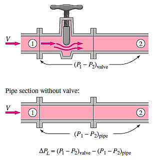
∆PL = (P1 – P2)value - (P1 – P2)Pipe
- Valves
- Couplings

In a fully developed turbulent pipe flow, the friction factor is determined by the Reynolds number and relative roughness  , which is the ratio of the pipe's mean height of roughness to its diameter. All published results are acquired from tedious experiments employing intentionally roughened surfaces (typically by gluing sand grains of a given size on the inner surfaces of the pipes), and the functional form of this dependence cannot be obtained from a theoretical study.
The friction factor was determined using the flow rate and pressure drop readings.
Curve-fitting experimental data yielded tabular, graphical, and functional results, which are presented in tabular, graphical, and functional formats.
The Colebrook equation was created when Cyril.F. Colebrook (1910–1997) integrated the existing data for transition and turbulent flow in smooth and rough pipes into the following implicit relation.

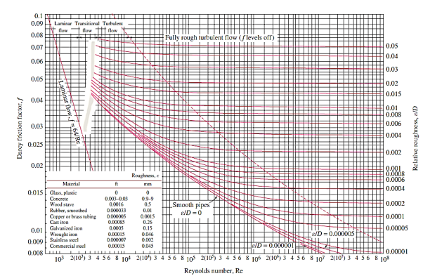
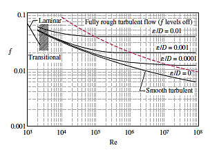
Lewis F. Moody (1880–1953) redrew Rouse's diagram into the current format two years later. It is given the now-famous Moody chart. It plots the Darcy friction factor for pipe flow as a function of Reynolds number and e/D over a wide range of Reynolds numbers and  values. It is one of the most extensively accepted and utilised engineering diagrams. Although it was designed for circular pipes, it can be used for noncircular pipes by substituting the hydraulic diameter for the diameter.
Commercially available pipes differ from those used in the trials in that their roughness is not uniform, making it impossible to give an exact description. Table and the Moody chart both show equivalent roughness levels for several commercial pipes.
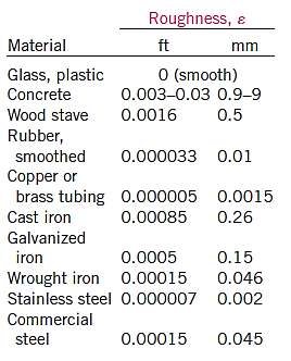
However, keep in mind that these figures are for fresh pipes, and as a result of corrosion, scale building, and precipitation, the relative roughness of pipes can rise over time. As a result, the friction factor could rise by 5 to 10 times. The design of piping systems must take into account actual operating circumstances. Furthermore, the Moody chart and its equivalent Colebrook equation are subject to a number of uncertainties (roughness size, experimental error, data curve fitting, and so on), therefore the findings produced should not be considered "precise." It's usually thought to be accurate to within  percent of the figure's range.
Because the Colebrook equation is implicit in f, iteration is required to determine the friction factor unless an equation solver such as EES is utilised. S. E. Haaland published an approximate explicit relation for f in 1983.

The findings derived from this relationship are within 2% of the Colebrook equation's results. When using a programmable calculator or a spreadsheet to solve for f with the equation, can be utilised as a good first guess in a Newton iteration if more exact results are required.
We make the following observations from the Moody chart:
- The friction factor for laminar flow decreases with rising Reynolds number and is unaffected by surface roughness.
- For a smooth pipe, the friction factor is lowest (although not zero because of the no-slip condition) and increases with roughness. In this scenario, the Colebrook equation ε = 0 reduces to the Prandtl equation.

- The shaded area in the Moody chart indicates the transition region from the laminar to turbulent regime (2300 < Re < 4000). Depending on flow disturbances, the flow in this region may be laminar or turbulent, or it may alternate between laminar and turbulent, causing the friction factor to fluctuate between values for laminar and turbulent flow. The information in this range is the least trustworthy. The friction factor increases in the transition area with modest relative roughness’s and approaches the value for smooth pipes.
- The friction factor curves corresponding to specified relative roughness curves are almost horizontal at very large Reynolds numbers (to the right of the dashed line in the chart), and hence the friction factors are independent of the Reynolds number. Because the thickness of the viscous sublayer drops with rising Reynolds number, it gets so thin that it is negligible in comparison to the surface roughness height, the flow in that region is referred to as fully rough, turbulent flow or simply fully rough flow. In this situation, the protruding roughness elements cause the viscous effects in the main flow, while the contribution of the laminar sublayer is insignificant.
- In the fully rough zone, the Colebrook equation reduces to the von Kármán equation stated as, which is clear in f. Although some publications refer to this zone as having wholly (or completely) turbulent flow, this is misleading because the flow to the left of the dashed blue line is likewise completely turbulent.

Key Takeaway:


Pipes in Series:
- When the pipes of different lengths and diameters are connected to each other to form a pipeline then such a pipeline is called as a compound pipe or pipes in series.
- As the pipes are in series, the discharge through each pipe will be same (continuous)
∴ Q = A1 V1 = A2 V2 = A3V3
- If a pipeline connecting two reservoirs by compound pipes, then the difference in liquid surface level is equal to the sum of the head losses in all the sections.
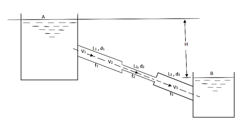
Let Q = Discharge through pipeline
H = Total loss of head
d₁ = Diameter of pipe 1
L₁ = Length of pipe 1
f₁ = Darcy's coefficient of friction
d2, L2, f2 =Corresponding value of pipe 2,
d3, L3, f3 =Corresponding value of pipe 3.
1. Considering all losses,
Total loss of head = Major losses + Minor losses
H=
∴Major losses = Head loss due to friction in each pipe

= 
∴Minor losses = Entrance loss+ Contraction loss+ Expansion loss+ Exit loss

2. If minor losses are neglected, then Total loss of head = Major losses
H = 1/2g [ 
3. If discharge through the pipe is given, then
H=[ 
Pipes in Parallel:
- When a pipeline divides into two or more parallel pipes which again join together at downstream as shown in Fig., then that pipe is said to be in parallel.
- In order to increase the discharge passing through the main pipe, the pipes are connected in parallel.
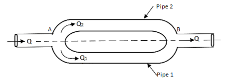
- The discharge in the main pipe is equal to sum of the discharge in each of the parallel pipes.
∴Q =Q1 + Q2
- When the pipes are arranged in parallel, the loss of head in each parallel pipe is same.
hf 1 = hf 2

Key Takeaways:
- When the pipes of different lengths and diameters are connected to each other to form a pipeline then such a pipeline is called as a compound pipe or pipes in series.
- When a pipeline divides into two or more parallel pipes which again join together at downstream as shown in Fig., then that pipe is said to be in parallel.
A syphon is a long-bent pipe is used for carrying water from a reservoir at a higher level to another reservoir at a lower level when the two reservoirs are separated by a hill or high-level ground.
The point C is highest point of syphon is called as summit.
The pressure at point C is less than atmospheric pressure as it lies above the free water surface in the tank A.
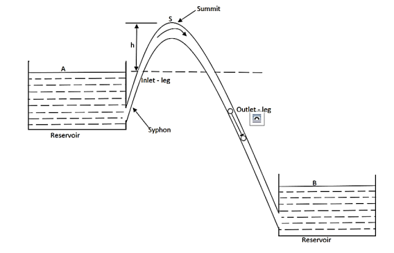
Fig: Siphon
The pressure at C can be reduced, theoretically, to -10.3 m of water but in actual practice is only 7.6 m of water (or 10.3-7.6=2.7 m of water absolute).
If the pressure becomes less than 2.7 m of water absolute, the dissolve air and other gases would come out from water and collected at the summit. It may be obstructed the flow of water.
Syphon is used in following cases:
(a) To take out water from one reservoir to another reservoir separated by a hill or ridge.
(b) To drain out water from a channel without any outlet.
(c) To take out the water from a tank which does not have any outlet.
Working principle of syphon:
Negative or vacuum pressure is created in the syphon, so that liquid gets pushed into it.
The flow through syphon then remains continuous till pressure in syphon pipe remains negative but less than separation pressure.
At summit, we find the minimum pressure. Velocity or discharge through syphon can be obtained by applying Bernoulli's equation between A and Fig.as shown in.
Now applying Bernoulli's equation between section A and B,
 +ZA=
+ZA= +ZB+Losses
But  and VA=VB=0
∴ZA-ZB=Losses
H= Loss of head at entry+ Head loss due to friction+ Head loss due to exit
H= 0.5 
Where f= Friction factor=4f=4 coefficient of friction
L = Length of syphon AB
d =Diameter of the syphon
V =Velocity of flow
Now, applying Bernoulli's equation between A and C.
 +ZA=
+ZA= +ZB+Losses between AC
But  =0, VA=0, Vc=V,
Head loss between AC=Entry loss +Frictional loss
=0.5 
∴ZA= 

But ZA-ZC=-hc
 = - [ hc + ( 1.5 +
This equation is used to find out,
 =Pressure head at summit
Hc = Height of summit above the surface in the higher level
L1= Length of inlet leg
Key Takeaway
- A syphon is a long-bent pipe is used for carrying water from a reservoir at a higher level to another reservoir at a lower level when the two reservoirs are separated by a hill or high-level ground.
- At summit, we find the minimum pressure. Velocity or discharge through syphon can be obtained by equation
Pressure head at summit  = - [ hc + ( 1.5 +
Power is transmitted through pipe by allowing water to flow through a pipe.
Now consider a pipe AB connected to a tank as shown it.
Let,
H = Head of water at inlet
L = Length of the pipe
d = Diameter of the pipe
V = Velocity of flow in pipe
hf =Head loss due to friction
Head available at the outlet of the pipe,
=Head at inlet-Head loss due to friction
= H-hf =H - 
Weight of water flowing through pipe/sec.
W =ρg x Volume of water/sec.
= ρg x Area× Velocity= ρg ×π/4 d2×V
Power transmitted at outlet of the pipe,
P = Weight of water per sec x Head at outlet
P= (ρg ×π/4 d2×V) [H -  Watt
Watt
Efficiency of power transmitted,
ɳ = 
=
= 
ɳ = 
Condition for Maximum Transmission of Power:
The condition for maximum transmission of power is obtained by differentiating Equation with respect to V and equating the same to zero.
∴ (P)=0
(P)=0
 (ρg ×π/4 d2×V) [H -
ρg ×π/4 d2 (H - 
H = 
∴hf=H/3
The Equation is the condition for maximum transmission of power.
Maximum Efficiency of Transmission of Power:
Efficiency of power transmission through pipe is given by,
ɳ=
For maximum power transmission, hf=H/3
Maximum efficiency,
ɳ= =2/3
=2/3
∴ɳ%=66.67%
Key Takeaway
- Power Transmitted = ρg ×π/4 d2×V
- Condition for Maximum Transmission of Power: hf=H/3
- Efficiency ɳ=

- Maximum efficiency, ɳ=
 =2/3=66.67%
We make use of dimensional analysis for three prominent reasons:
- To check the consistency of a dimensional equation.
- To derive the relation between physical quantities in physical phenomena.
- To change units from one system to another.
Understanding dimensions is of utmost importance as it helps us in studying the Nature of physical quantities mathematically. The basic concept of dimensions is that we can add or subtract only those quantities which have same dimensions. Also, two physical quantities are equal if they have same dimensions.
Dimensional analysis is a mathematical technique used to predict physical parameters that influence the flow in fluid mechanics, heat transfer in thermodynamics, and so forth. The analysis involves the fundamental units of dimensions MLT: mass, length, and time.
A typical fluid mechanics problem typical fluid mechanics problem in which experimentation is required consider the experimentation is required consider the steady flow of an steady flow of an incompressible Newtonian fluid through a long, smooth incompressible Newtonian fluid through a long, smooth walled, horizontal, circular pipe.
The first step in the planning of an experiment to study this problem would be to decide the factors, or variables, that will have an effect on the pressure drop.
Pressure drop per unit length p f ( D , , , V )
Key Takeaway:
- Pressure drop per unit length depends on FOUR variables: sphere size (D); speed (V); fluid density ( ρ); fluid viscosity ().
- A physical equation is the relationship between two or more physical quantities.
- Any correct equation expressing a physical relationship between quantities must be dimensionally homogeneous and numerically equivalent.
- Dimensional homogeneity states that every term in an equation when reduced to fundamental dimensions must contain identical powers of each dimension.
- A dimensionally homogeneous equation is applicable to all system of units.
- In a dimensionally homogeneous equation, only quantities having the same dimensions can be added, subtracted or equated.
P = w h
Dimensions of LHS = ML-1T-2
Dimensions of RHS = ML-2T-2×L = ML-1T-2
Dimensions of LHS = Dimensions of RHS
Hence, equation P= w h is dimensionally homogeneous; so it can be used in any system of units.
Applications of Dimensional Homogeneity:
- It facilitates to determine the dimensions of a physical quantity.
- It helps to check whether an equation of a physical phenomenon is dimensionally homogeneous or not.
- It facilitates conversion of units from one system to another.
Key takeaways
- Dimensional homogeneity states that every term in an equation when reduced to fundamental dimensions must contain identical powers of each dimension.
- A dimensionally homogeneous equation is applicable to all system of units.
This method is used to find the expression for a variable that is dependent on no more than three or four variables. When the number of independent variables exceeds four, finding an expression for the dependent variable becomes quite difficult.
Let X is a variable, which depends on
X1, X2 & X3
Mathematically it is written as,
X = f [X1, X2 & X3]
It can also be written as,
X = KX1a, X2b & X3c
Where K = constant
a, b, c, are arbitrary Powers
Example: The length (L) of a pendulum and the acceleration due to gravity determine the time-period (t) of the pendulum (g). Determine a time-period expression.
Solution:
Time period (t) is a function of L & g
t = KLa. gb
Substituting the dimensions on both sides,
T1 = KLa(LT-2)b
Equating the powers of M, L and T on both sides, we have
Power of T, 1 = -2b, So, b = - ½
Power of L, 0 = a+b, So, a = 1/2
Substituting the values,
t = KLa.gb
t = KL1/2.g-1/2 = k √L/g
The value of K is determined from experiments which is given as,
K = 2π
t= 2π √L/g
Key Takeaway:
X = f [X1, X2 & X3]
X = KX1a, X2b & X3c
- When a large number of physical variables are involved Rayleigh’s method of dimensional analysis becomes increasingly laborious and cumbersome.
- Buckingham’s method is an improvement over the Rayleigh’s method.
- Buckingham’s designated the dimensionless group by the letter Π. It is therefore often called Buckingham Π-Method.
- The Buckingham’s Π-Method states as follows:
“If there are n variables in a dimensionally homogeneous equation and if these variables contain fundamental dimensions (such as M, L, T, etc.) then the variables are arranged into (n-m) dimensionless terms.
These dimensionless terms are called Π– terms.”
Mathematically, if any variable X1, depends on independent variables, X2, X3, X4,…… Xn; the functional equation may be written as
X1 = f [X2, X3, X4,…… Xn] -------- 1
Equation 1 can also be written as
f1 [X1, X2, X3,…… Xn] -------- 2
It is dimensionally homogeneous equation and contains n variables.
If there are m fundamental dimensions, then according to Buckingham’s Π– theorem, it can be written in terms of number of Π– terms in which number of Π terms is equal to (n-m).
Hence equation 2 becomes as
f1 [π1, π2, π3,…… πn-m] --------3
Each dimensionless π– term is formed by combining m variables out of the total n variables with one of the remaining (n-m) variable.
These m variables which appear repeated in each of π– terms are consequently called repeating variables and are chosen from among the variables such that they together involve all the fundamental dimensions and they themselves do not form a dimensionless parameter.
Let in the above case X2, X3 and X4 are the repeating variables if the fundamental dimensions m (M, L, T) = 3, then each term is written as:
π1 = X2a1, X3b1 & X4c1.X1
π2 = X2a2, X3b2 & X4c2.X5
.
.
.
πn-m =  -------- 4
Where a1, b1, c1, a2, b2, c2 etc. are the constants, which are determined by considering dimensional homogeneity. These values are substituted in equation 4 and values of π1, π2, π3,…… πn-m are obtained. These values of Π’s are substituted in equation 3.
The final general equation for the phenomenon may then be obtained by expressing anyone of the Π– terms as a function of the other as:
π1= ∅( π2, π3,…… πn-m)
π2= ∅( π1, π2,…… πn-m)
Key takeaways:
The final general equation for the phenomenon may then be obtained by expressing anyone of the Π– terms as a function of the other as:
π1= ∅( π2, π3,…… πn-m)
π2= ∅( π1, π2,…… πn-m)
Model: is the small-scale replica of the actual structure or machine. It is not necessary that models should be smaller than the prototypes (although in most of the cases it is), they may be larger than the prototypes.
Prototype: The actual structure or machine
Model analysis: the study of models of actual machine.
Advantages:
- The performance of the machine can be easily predicted, in advance.
- With the help of dimensional analysis, a relationship between the variables influencing a flow problem in terms of dimensional parameters is obtained. This relationship helps in conducting tests on the model.
- The merits of alternative designs can be predicted with the help of model testing. The most economical and safe design may be, finally, adopted.
Types of similarities between model and prototype - Three types of similarities must exist between the model and prototype.
Geometric Similarity:
The ratio of all corresponding linear dimension in the model and prototype are equal.
Let Lm = length of model
bm = width of model
dm = diameter of model
Am = area of model
Vm = volume of model
Lp, bp, dp, Ap, Vp are corresponding values of the prototype.


Key Takeaways:
- Model: is the small-scale replica of the actual structure or machine. It is not necessary that models should be smaller than the prototypes (although in most of the cases it is), they may be larger than the prototypes.
- With the help of dimensional analysis, a relationship between the variables influencing a flow problem in terms of dimensional parameters is obtained. This relationship helps in conducting tests on the model.
Similitude
- Similitude are concept that applies to the testing of engineering models. The model is said to resemble a real application if it has two geometric similarities, kinematic similarities and dynamic similarities. Similarities and Similitude are the alternate in this context.
- The term dynamic Similitude is often used to capture everything because it means that geometric and kinematic similarities have been met.
- Similitude's main application is in hydraulic and aerospace engineering to test fluid flow conditions with rated models. And it is the main idea behind many liquid formulas for liquid formulas.
- Engineering models are used to study the complex problems of fluid dynamics where computer calculations and simulations are unreliable. Models tend to be smaller than the final build, but not always. The types of scales allow for design testing before construction, and in many cases are critical step in the development process.
- The design of the scale model, however, must be accompanied by analysis to determine under which conditions it was tested. While geometry can be simply measured, other parameters, such as pressure, temperature or velocity and the type of liquid may need to be adjusted. Similarities are found when experimental conditions are created in such a way that test results apply to actual construction.
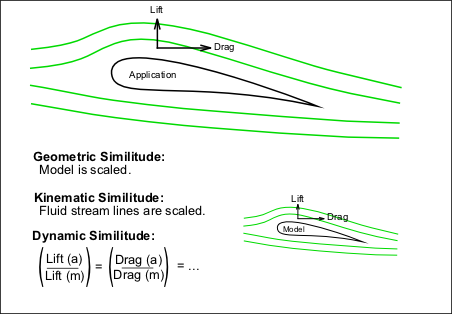
Fig: Three conditions are required for the model to match the system.
The following methods are needed to achieve similarity;
Geometric Similarity - the model is the same method as the system, which is usually measured.
Kinematic similarity - the fluid flow of both the model and the actual application must exceed the same levels of motion change time. (Liquid distribution is the same)
Dynamic similarity - the ratio of all forces acting on liquid-related particles and parameters in both systems remains the same.
To satisfy the above conditions the application is analyzed;
- All parameters required to define a system are identified using terms from the continuation mechanics.
- Quantitative analysis is used to present the system with as few independent variables and as many measurable parameters as possible.
- The non-measurable parameter values are held to be the same for all scale model and usage. This can be done because it is flawless and will ensure a strong similarity between the model and use. Emerging statistics are used to obtain measurement rules governing modular test conditions.
- It is often not possible to achieve strong similarities during model testing. The bigger the application, the harder it is to match. In these cases some of the features of the simulation are ignored, focusing only on the most important parameters.
- The construction of ships is often more sophisticated than science for the most part because the strong similarities are very difficult to find a slightly submerged vessel: the ship is affected by air forces in the air above it, by hydrodynamic forces inside the water beneath it, and especially by wave movements in the visible connection between water and air.
- The requirements for each of these scenarios vary, so the models cannot replicate what happens on a full-size vessel almost as much as a plane or submarine can - each works perfectly on the same object.
- Matching is a term widely used in fragmentation techniques related to the complex lifestyle. Under loading conditions provided fatigue damage to the excluded template can be compared to that of the excluded sample. The similarities suggest that the fatigue life of two people will also be the same.
Key takeaways
Similitude are concept that applies to the testing of engineering models. The model is said to resemble a real application if it has two geometric similarities, kinematic similarities and dynamic similarities. Similarities and Similitude are the alternate in this context.
The term dynamic Similitude is often used to capture everything because it means that geometric and kinematic similarities have been met.
References:
1. Introduction to Fluid Mechanics, James E.A., John and Haberm W.A., Prentice Hall of India
2. Fluid Mechanics, Jain A.K., Khanna Publication
3. Engineering Fluid Mechanics, Garde R.J. And MirajGoankar, Nemchand&Bros, Roorkee, SCITECH, Publication (India) Pvt. Ltd.
4. Fluid Mechanics and Fluid Power Engineering, Dr. D.S. Kumar, S.K. Kataria& sons
5. Fluid Mechanics, Frank M. White, McGraw Hill Publication