Unit - 2
Transfer Function system Representation through Block Diagram and Signal Flow Graph
Advantages of Block diagram reduction technique:
- Very simple to Construct the Block diagram of complicated electrical & mechanical systems.
- The function of individual element can be visualized form block diagram
- Individual as well as overall performance of the system can be studied by the figure shown in Block diag.
- Overall CLTF can be easily calculated by Block diagram reduction rules.
Disadvantages of Block diagram reduction technique:
It does not include any information above physical construct of system (completely mathematical approach). Source of energy is generally not shown in the block diagram so diff. Block diagram can be drawn for the same function.
CLTf: -ve feedback
C(s)/R(s)= G(s)/1+G(s)H(s)
CLTF:-+vefeedback
C(S)/R(S) = G(S)/1-G(s)H(S)
Rules of Block diagram Algebra:
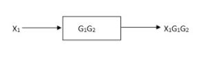
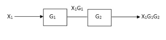
Block in cascade


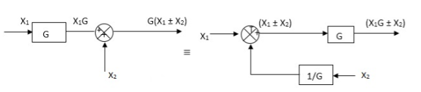
Moving summing point after a block
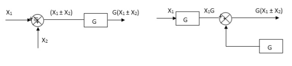
Moving summing point ahead of block

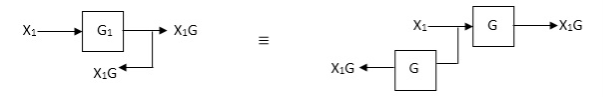
Moving take off point after a block
Moving take off point ahead a block

Eliminating a feedback Loop

Fig 1. Block Diagram Reduction Techniques
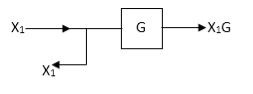
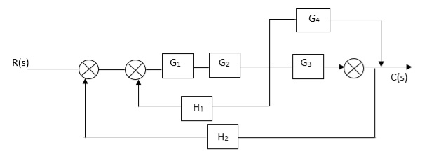
Q. Reduce given B.D to canonical (simple form) and hence obtain the equivalent Tf = c(s)/ R(S)?

Sol:

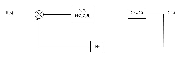

Fig 2. Final reduced block diagram
C(S)/R(S) = (G1G2) (G3+G4)/1+G1G2H1)/1-G1,G2(G3+G4) H2/1+G1G2H1
= G1G2(G3+G4)/1+G1G2H1-G1G2H2(G3+G4)
=G1G2(G3+G4)/1+(H1-H2)(G1G2) (G3+G4)
C(s)/R(S) = G1G2(G3+G4)/1+(H1-H2(G3+G4)) G1 G2
Q) Reduce the Block diagram
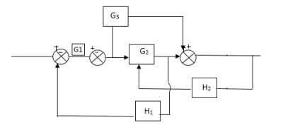
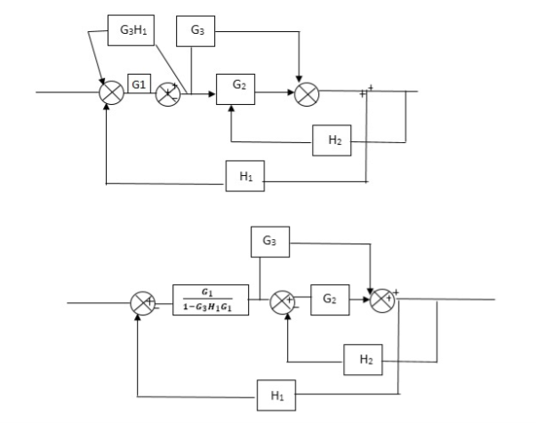

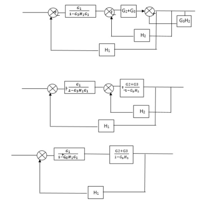

Fig 3. Final Reduced Block diagram
C(s)/R(s)= G1(G3+G2)/(1-G1G3X1) (1-G2X2) H1
= G(G3+G2)/(1-G3G1H1) (1-G2H2) + G1H1(G3+G2)
= G1(G3+G2)/1-63G1H1-G2H2+G1H1(G3+G2H1
=G1(G3+G2)/1-G3H2+G1G2H1(1+G3H2)
As we already know that Block Diagram is represented as shown below
SFG

RULES:
1) The signal travels along a branch in the direction of an arrow.
2) The lip signal is multiplied by the transmittance to obtain the o/p.
3) I/p signal at a node is sum of all the signals entering at that node.
4) A node transmits signal at all branches leaving that node.
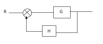
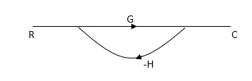
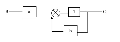
Q: For given block diagram draw the SFG?


Ra+cb =c
c/R= a/1-b
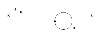
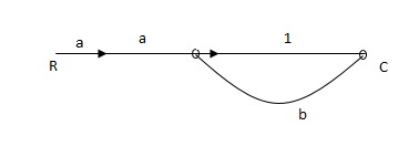
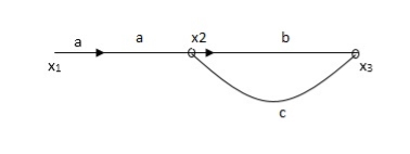
Q. The SFG shown has forward path and singles isolated loop determine overall transmittance relating X3 and X1?

Sol:
X1- I/p node
X2-Intenmediale node
X3- o/p node
Ab- forward path (p)
Bc- 1 loop (L)
At node XQ:
X2 = x1a + x3c [Add i/p signals at node]
At node x3:
x2b =x3
(x1a+x3c) b = x3
X1ab = x3 (1-bc)
X1 = x3 (1-bc)/ab
Ab/(1-bc) = x3/x1
T= p/1-L

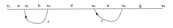
X1:- I/p node x2, x3,x4,x5,Qnlexmedili node
X0:- o/p node abdeg:- forward path
Bc, ef :- Loop [isolated]
x2 = ax1+c x3
x3= bx2
x4 = d x3+f x5
x5 = e x4
x6= g x5
x6 = g(e x4) = ge [dx3+ e f x5]
xb = ge [d (bx2) + f (e x4)]
xb = ge [ db (ax1+cx3) + fe (dx3+ fx5)]
xb = ge [db (ax1+cb (ax1+x3) +fe[cdbx2]+
f( e [db (ax1+ cx3)
x2 = ax1 + cb (x2) x4 = d bx2 + f exq
x2 = ax1 + cbx2 = db (d4) + fe/1-cb
x2 = ax1/(1-cb) xy = db x2 + f x6/g
xy = db [ax1]/1-cb + f xb/g
x5 = c db( ax1)/1-cb + efxb/g
xb = gx5
= gedb (ax1)/1-cb + g efxb/g
Xb = gx5
Gedb (ax1)/1-cb + g efxb/g
(1- gef/g) xb = gedb ax1/1-ab
Xb/x1 = gedb a/ (1- ef – bc + beef
Xb/x1 = p/ 1- (L1+L2) + L1 L2 for isolated loops
An Observable canonical form is used to analyse and design control systems because this form allows observability. A system is observable if all its states can be determined by the output. Consider a transfer function of third order
 =T(s)=(b0s3+b1s2+b2s+b3)/(s3+a1s2+a2s+a3)
T(s)=(b0+b1/s+b2s2+b3/s3)/[1-(-a1/s-a2/s2-a3/s3)] …………(1)
By Mason’s Gain Formula
T= …………(2)
Pk forward path transmittance of k+n path from a specified i/p node to n o/p nodes
While calculating ipnode to n o/p nodes.
 it is the graphics determined which involves of transmittances and multiple increases b/w non touching loops.
 = 1- [sum of all individual loop transmitting]
+[ sum of loop transmittance product of all possible non- touching loops]
-[sum of loop transmittance of all possible triples of non- touching loops]
 path factor associated with concered path & involves all a in the graphic which are isolated from forward path under consideration.
The path factor  for kthis equal to graph determinant of SFG which effect after erasing the kth path from the graph.
The required SFG is shown below, we can conclude
y=x1+b0u
 =-a1(x1+b0u)+x2+b1u
=-a1x1+x2+(b1-a1b0)u ……….(3)
 =-a2x1+x3+(b2-a2b0)u ……….(4)
 =-a3x1+(b3-a3b0)u …………(5)
y=[1 0 0] +b0u ………….(6)
The resulting matrix is given below
The above equations in matrix form can be easily interpreted through the signal flow graph. From the equation (3) and (5) we can say that
a) There are three feedback loops touching each other and having gain -a1/s, -a2/s2 and -a3/s3.
b) There are four forward paths touching the loop and having gain b0, b1/s, b2/s2, b3/s3.
So, the signal flow graph is shown below

Fig 4: SFG for observable Form
Question: Find the observable canonical realization of the system H(s)=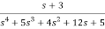
Solution: The above transfer function can be also written as
H(s)=
Comparing above equation with standard equation we conclude that
The gains of forward paths are 
The feedback loop gains are 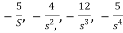
The SFG satisfying above conditions will be

The observable canonical form can be obtained by converting the above SFG to block diagram

Fig 5. Observable canonical form can be obtained by converting the above SFG to block diagram
Controllable Canonical Form: In this the transfer function is divided into two parts as shown in below figure.

Fig 6: A third order system

Fig 7: Simplified representation of above system
G(s)= =
= 
 =
= ………..(7)
 =b0s3+b1s2+b2s+b3
The equation relating phase variable to input is given as
The equation relating output to phase variable can be given as(refer eq.(7))
y=b0 +b1
+b1 +b1
+b1 +b3x1
+b3x1
=b0(-a3x1-a2x2-a1x3+u)+b1x3+b2x2+b3x1
=(b3-a3b0)x1+(b2-a2b0)x2+(b1-a1b0)x3+b0u
The above equation in vector matrix form can be written as
y=[((b3-a3b0) (b2-a2b0) (b1-a1b0)] +b0u ……..(8)
The signal flow graph for above vector matrix equations is shown below

Fig 8: SFG for controllable form
Key takeaway
i) Matrix A is known as Bush form or companion form. Matrix B has all elements zero except the last element.
Ii) A system is observable if all its states can be determined by the output
Question: Find the controllable canonical realization of the following systems
a) H(s)=
b) H(s)=
Solution: a)H(s)=
Let H(s)=
 =
=
H1(s)= 1/s+6
1/s+6
X(s)=sX1(s)+6X1(s)
SX1(s)=X(s)+6X1(s)
We can get X1(s) by passing sX1(s) through integrator. The above equation can be realised as

Fig 9. H1(s)= 1/s+6
1/s+6
H2(s)= s+2
s+2
Similarly, Y(s)=sX1(s)+2X1(s)
H2(s)= s+2
s+2

Fig 10. H2(s)= s+2
s+2
The complete realization of transfer function can be obtained by combining the above two realizations. The complete realization will be
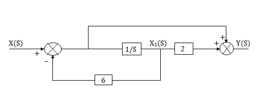
Fig 11. Complete realization of H(s)=
b)H(s)=
Let H(s)= =
= 
 =s+3
=s+3
Y(s)=sX1(s)+3X1(s)
The above transfer function can be realised as
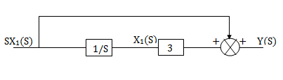
Fig 12.  =s+3
=s+3
Now,  =
=
s2X1(s)=X(s)-2sX1(s)-5X1(s)
Assuming s2X1(s) is available the above transfer function can be realised as

Fig 13.  =
=
The complete realization of transfer function can be obtained by combining the above two realizations. The complete realization will be

Fig 14. H(s)=
T= 
The overall transmittance Coverall gain can be determined by Masks formula.
Explanation
Pk forward path transmittance of k+n path from a specified i/p node to n o/p nods
While calculating ip node to n o/p nods.
While calculating ip no node should be encountered (used) more than ones.
 it is the graphics determined which involves of transmittances and multiple increases b/w non touching loops.
 = 1- [sum of all individual loop transmitting]
+[ sum of loop transmittance product of all possible non- touching loops]
-[sum of loop transmittance of all possible triples of non- touching loops]
 path factor associated with concered path & involves all a in the graphic which are isolated from forward path under consideration.
The path factor  for kthis equal to graph determinant of SFG which effect after erasing the kth path from the graph
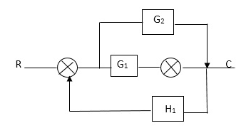
Q. Draw SFG for given block diagram?

Sol:

P1= G1 p2 =G2 Delta1 =1
L1= -G1 H1
 = 1-(-G1H1)
= 1+G1H1
T= G1+G2/1+G1H1
Q: Determine overall gain x5 and x1 Draw SFG
X2 = ax1+ f x2
X3= bx2 +exy
X4 = cx3+hx5
X5 =dx4 + gx2

P1 = abcd p2 = ag
L1 = f L2 = ce, L3= dh
 1 = 1
1 = 1
 2= 1-ce
 = 1-[L2+L2+L3] + [L1 L2 +L1 L3]
= 1-[f+ le = dh] + [fce +fdh]
T= abcd+ ag (1-ce)/1-[ftce + dh ] + (fce + fdh)
Key takeaway
- The function of individual element can be visualized from block diagram
- The signal travels along a branch in the direction of an arrow.
- The input signal is multiplied by the transmittance to obtain the o/p.
References:
1. I. J. Nagrath and M. Gopal, “Control Systems Engineering”, New Age International, 2009.
2. K. Ogata, “Modern Control Engineering”, Prentice Hall, 1991
3. M. Gopal, “Control Systems: Principles and Design”, McGraw Hill Education, 1997.
4. B. C. Kuo, “Automatic Control System”, Prentice Hall, 1995.
Unit - 2
Transfer Function system Representation through Block Diagram and Signal Flow Graph
Advantages of Block diagram reduction technique:
- Very simple to Construct the Block diagram of complicated electrical & mechanical systems.
- The function of individual element can be visualized form block diagram
- Individual as well as overall performance of the system can be studied by the figure shown in Block diag.
- Overall CLTF can be easily calculated by Block diagram reduction rules.
Disadvantages of Block diagram reduction technique:
It does not include any information above physical construct of system (completely mathematical approach). Source of energy is generally not shown in the block diagram so diff. Block diagram can be drawn for the same function.
CLTf: -ve feedback
C(s)/R(s)= G(s)/1+G(s)H(s)
CLTF:-+vefeedback
C(S)/R(S) = G(S)/1-G(s)H(S)
Rules of Block diagram Algebra:
Block in cascade


Moving summing point after a block

Moving summing point ahead of block

Moving take off point after a block

Moving take off point ahead a block
Eliminating a feedback Loop
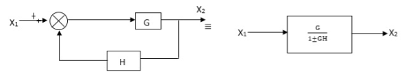
Fig 1. Block Diagram Reduction Techniques
Q. Reduce given B.D to canonical (simple form) and hence obtain the equivalent Tf = c(s)/ R(S)?

Sol:
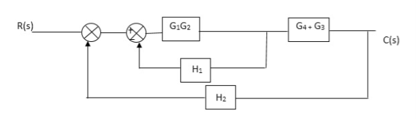

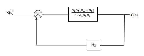
Fig 2. Final reduced block diagram
C(S)/R(S) = (G1G2) (G3+G4)/1+G1G2H1)/1-G1,G2(G3+G4) H2/1+G1G2H1
= G1G2(G3+G4)/1+G1G2H1-G1G2H2(G3+G4)
=G1G2(G3+G4)/1+(H1-H2)(G1G2) (G3+G4)
C(s)/R(S) = G1G2(G3+G4)/1+(H1-H2(G3+G4)) G1 G2
Q) Reduce the Block diagram


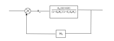
Fig 3. Final Reduced Block diagram
C(s)/R(s)= G1(G3+G2)/(1-G1G3X1) (1-G2X2) H1
= G(G3+G2)/(1-G3G1H1) (1-G2H2) + G1H1(G3+G2)
= G1(G3+G2)/1-63G1H1-G2H2+G1H1(G3+G2H1
=G1(G3+G2)/1-G3H2+G1G2H1(1+G3H2)
As we already know that Block Diagram is represented as shown below

SFG
RULES:
1) The signal travels along a branch in the direction of an arrow.
2) The lip signal is multiplied by the transmittance to obtain the o/p.
3) I/p signal at a node is sum of all the signals entering at that node.
4) A node transmits signal at all branches leaving that node.
Q: For given block diagram draw the SFG?


Ra+cb =c
c/R= a/1-b
Q. The SFG shown has forward path and singles isolated loop determine overall transmittance relating X3 and X1?
Sol:
X1- I/p node
X2-Intenmediale node
X3- o/p node
Ab- forward path (p)
Bc- 1 loop (L)
At node XQ:
X2 = x1a + x3c [Add i/p signals at node]
At node x3:
x2b =x3
(x1a+x3c) b = x3
X1ab = x3 (1-bc)
X1 = x3 (1-bc)/ab
Ab/(1-bc) = x3/x1
T= p/1-L

X1:- I/p node x2, x3,x4,x5,Qnlexmedili node
X0:- o/p node abdeg:- forward path
Bc, ef :- Loop [isolated]
x2 = ax1+c x3
x3= bx2
x4 = d x3+f x5
x5 = e x4
x6= g x5
x6 = g(e x4) = ge [dx3+ e f x5]
xb = ge [d (bx2) + f (e x4)]
xb = ge [ db (ax1+cx3) + fe (dx3+ fx5)]
xb = ge [db (ax1+cb (ax1+x3) +fe[cdbx2]+
f( e [db (ax1+ cx3)
x2 = ax1 + cb (x2) x4 = d bx2 + f exq
x2 = ax1 + cbx2 = db (d4) + fe/1-cb
x2 = ax1/(1-cb) xy = db x2 + f x6/g
xy = db [ax1]/1-cb + f xb/g
x5 = c db( ax1)/1-cb + efxb/g
xb = gx5
= gedb (ax1)/1-cb + g efxb/g
Xb = gx5
Gedb (ax1)/1-cb + g efxb/g
(1- gef/g) xb = gedb ax1/1-ab
Xb/x1 = gedb a/ (1- ef – bc + beef
Xb/x1 = p/ 1- (L1+L2) + L1 L2 for isolated loops
An Observable canonical form is used to analyse and design control systems because this form allows observability. A system is observable if all its states can be determined by the output. Consider a transfer function of third order
 =T(s)=(b0s3+b1s2+b2s+b3)/(s3+a1s2+a2s+a3)
T(s)=(b0+b1/s+b2s2+b3/s3)/[1-(-a1/s-a2/s2-a3/s3)] …………(1)
By Mason’s Gain Formula
T= …………(2)
Pk forward path transmittance of k+n path from a specified i/p node to n o/p nodes
While calculating ipnode to n o/p nodes.
 it is the graphics determined which involves of transmittances and multiple increases b/w non touching loops.
 = 1- [sum of all individual loop transmitting]
+[ sum of loop transmittance product of all possible non- touching loops]
-[sum of loop transmittance of all possible triples of non- touching loops]
 path factor associated with concered path & involves all a in the graphic which are isolated from forward path under consideration.
The path factor  for kthis equal to graph determinant of SFG which effect after erasing the kth path from the graph.
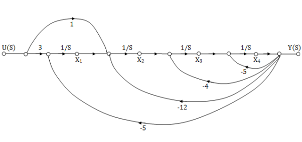
The required SFG is shown below, we can conclude
y=x1+b0u
 =-a1(x1+b0u)+x2+b1u
=-a1x1+x2+(b1-a1b0)u ……….(3)
 =-a2x1+x3+(b2-a2b0)u ……….(4)
 =-a3x1+(b3-a3b0)u …………(5)
y=[1 0 0] +b0u ………….(6)
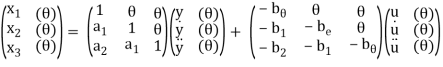
The resulting matrix is given below

The above equations in matrix form can be easily interpreted through the signal flow graph. From the equation (3) and (5) we can say that
a) There are three feedback loops touching each other and having gain -a1/s, -a2/s2 and -a3/s3.
b) There are four forward paths touching the loop and having gain b0, b1/s, b2/s2, b3/s3.
So, the signal flow graph is shown below

Fig 4: SFG for observable Form
Question: Find the observable canonical realization of the system H(s)=
Solution: The above transfer function can be also written as
H(s)=
Comparing above equation with standard equation we conclude that
The gains of forward paths are 
The feedback loop gains are 
The SFG satisfying above conditions will be
The observable canonical form can be obtained by converting the above SFG to block diagram

Fig 5. Observable canonical form can be obtained by converting the above SFG to block diagram
Controllable Canonical Form: In this the transfer function is divided into two parts as shown in below figure.

Fig 6: A third order system
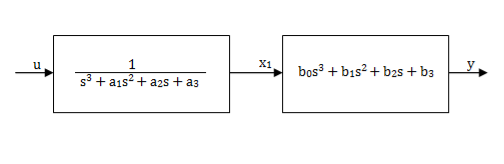
Fig 7: Simplified representation of above system
G(s)= =
= 
 =
= ………..(7)
 =b0s3+b1s2+b2s+b3
The equation relating phase variable to input is given as

The equation relating output to phase variable can be given as(refer eq.(7))
y=b0 +b1
+b1 +b1
+b1 +b3x1
+b3x1
=b0(-a3x1-a2x2-a1x3+u)+b1x3+b2x2+b3x1
=(b3-a3b0)x1+(b2-a2b0)x2+(b1-a1b0)x3+b0u
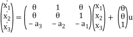
The above equation in vector matrix form can be written as
y=[((b3-a3b0) (b2-a2b0) (b1-a1b0)] +b0u ……..(8)
The signal flow graph for above vector matrix equations is shown below

Fig 8: SFG for controllable form
Key takeaway
i) Matrix A is known as Bush form or companion form. Matrix B has all elements zero except the last element.
Ii) A system is observable if all its states can be determined by the output
Question: Find the controllable canonical realization of the following systems
a) H(s)=
b) H(s)=
Solution: a)H(s)=
Let H(s)=
 =
=
H1(s)= 1/s+6
1/s+6
X(s)=sX1(s)+6X1(s)
SX1(s)=X(s)+6X1(s)
We can get X1(s) by passing sX1(s) through integrator. The above equation can be realised as
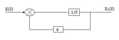
Fig 9. H1(s)= 1/s+6
1/s+6
H2(s)= s+2
s+2
Similarly, Y(s)=sX1(s)+2X1(s)
H2(s)= s+2
s+2
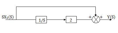
Fig 10. H2(s)= s+2
s+2
The complete realization of transfer function can be obtained by combining the above two realizations. The complete realization will be

Fig 11. Complete realization of H(s)=
b)H(s)=
Let H(s)= =
= 
 =s+3
=s+3
Y(s)=sX1(s)+3X1(s)
The above transfer function can be realised as

Fig 12.  =s+3
=s+3
Now,  =
=
s2X1(s)=X(s)-2sX1(s)-5X1(s)
Assuming s2X1(s) is available the above transfer function can be realised as

Fig 13.  =
=
The complete realization of transfer function can be obtained by combining the above two realizations. The complete realization will be

Fig 14. H(s)=
T= 
The overall transmittance Coverall gain can be determined by Masks formula.
Explanation
Pk forward path transmittance of k+n path from a specified i/p node to n o/p nods
While calculating ip node to n o/p nods.
While calculating ip no node should be encountered (used) more than ones.
 it is the graphics determined which involves of transmittances and multiple increases b/w non touching loops.
 = 1- [sum of all individual loop transmitting]
+[ sum of loop transmittance product of all possible non- touching loops]
-[sum of loop transmittance of all possible triples of non- touching loops]
 path factor associated with concered path & involves all a in the graphic which are isolated from forward path under consideration.
The path factor  for kthis equal to graph determinant of SFG which effect after erasing the kth path from the graph
Q. Draw SFG for given block diagram?
Sol:
P1= G1 p2 =G2 Delta1 =1
L1= -G1 H1
 = 1-(-G1H1)
= 1+G1H1
T= G1+G2/1+G1H1
Q: Determine overall gain x5 and x1 Draw SFG
X2 = ax1+ f x2
X3= bx2 +exy
X4 = cx3+hx5
X5 =dx4 + gx2
P1 = abcd p2 = ag
L1 = f L2 = ce, L3= dh
 1 = 1
1 = 1
 2= 1-ce
 = 1-[L2+L2+L3] + [L1 L2 +L1 L3]
= 1-[f+ le = dh] + [fce +fdh]
T= abcd+ ag (1-ce)/1-[ftce + dh ] + (fce + fdh)
Key takeaway
- The function of individual element can be visualized from block diagram
- The signal travels along a branch in the direction of an arrow.
- The input signal is multiplied by the transmittance to obtain the o/p.
References:
1. I. J. Nagrath and M. Gopal, “Control Systems Engineering”, New Age International, 2009.
2. K. Ogata, “Modern Control Engineering”, Prentice Hall, 1991
3. M. Gopal, “Control Systems: Principles and Design”, McGraw Hill Education, 1997.
4. B. C. Kuo, “Automatic Control System”, Prentice Hall, 1995.
Unit - 2
Transfer Function system Representation through Block Diagram and Signal Flow Graph
Advantages of Block diagram reduction technique:
- Very simple to Construct the Block diagram of complicated electrical & mechanical systems.
- The function of individual element can be visualized form block diagram
- Individual as well as overall performance of the system can be studied by the figure shown in Block diag.
- Overall CLTF can be easily calculated by Block diagram reduction rules.
Disadvantages of Block diagram reduction technique:
It does not include any information above physical construct of system (completely mathematical approach). Source of energy is generally not shown in the block diagram so diff. Block diagram can be drawn for the same function.
CLTf: -ve feedback
C(s)/R(s)= G(s)/1+G(s)H(s)
CLTF:-+vefeedback
C(S)/R(S) = G(S)/1-G(s)H(S)
Rules of Block diagram Algebra:
Block in cascade


Moving summing point after a block

Moving summing point ahead of block
Moving take off point after a block

Moving take off point ahead a block

Eliminating a feedback Loop

Fig 1. Block Diagram Reduction Techniques
Q. Reduce given B.D to canonical (simple form) and hence obtain the equivalent Tf = c(s)/ R(S)?
Sol: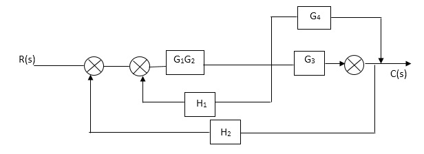


Fig 2. Final reduced block diagram
C(S)/R(S) = (G1G2) (G3+G4)/1+G1G2H1)/1-G1,G2(G3+G4) H2/1+G1G2H1
= G1G2(G3+G4)/1+G1G2H1-G1G2H2(G3+G4)
=G1G2(G3+G4)/1+(H1-H2)(G1G2) (G3+G4)
C(s)/R(S) = G1G2(G3+G4)/1+(H1-H2(G3+G4)) G1 G2
Q) Reduce the Block diagram


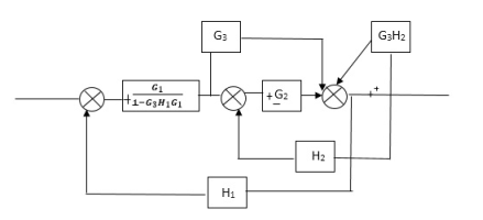


Fig 3. Final Reduced Block diagram
C(s)/R(s)= G1(G3+G2)/(1-G1G3X1) (1-G2X2) H1
= G(G3+G2)/(1-G3G1H1) (1-G2H2) + G1H1(G3+G2)
= G1(G3+G2)/1-63G1H1-G2H2+G1H1(G3+G2H1
=G1(G3+G2)/1-G3H2+G1G2H1(1+G3H2)
As we already know that Block Diagram is represented as shown below

SFG

RULES:
1) The signal travels along a branch in the direction of an arrow.
2) The lip signal is multiplied by the transmittance to obtain the o/p.
3) I/p signal at a node is sum of all the signals entering at that node.
4) A node transmits signal at all branches leaving that node.
Q: For given block diagram draw the SFG?


Ra+cb =c
c/R= a/1-b
Q. The SFG shown has forward path and singles isolated loop determine overall transmittance relating X3 and X1?

Sol:
X1- I/p node
X2-Intenmediale node
X3- o/p node
Ab- forward path (p)
Bc- 1 loop (L)
At node XQ:
X2 = x1a + x3c [Add i/p signals at node]
At node x3:
x2b =x3
(x1a+x3c) b = x3
X1ab = x3 (1-bc)
X1 = x3 (1-bc)/ab
Ab/(1-bc) = x3/x1
T= p/1-L
X1:- I/p node x2, x3,x4,x5,Qnlexmedili node
X0:- o/p node abdeg:- forward path
Bc, ef :- Loop [isolated]
x2 = ax1+c x3
x3= bx2
x4 = d x3+f x5
x5 = e x4
x6= g x5
x6 = g(e x4) = ge [dx3+ e f x5]
xb = ge [d (bx2) + f (e x4)]
xb = ge [ db (ax1+cx3) + fe (dx3+ fx5)]
xb = ge [db (ax1+cb (ax1+x3) +fe[cdbx2]+
f( e [db (ax1+ cx3)
x2 = ax1 + cb (x2) x4 = d bx2 + f exq
x2 = ax1 + cbx2 = db (d4) + fe/1-cb
x2 = ax1/(1-cb) xy = db x2 + f x6/g
xy = db [ax1]/1-cb + f xb/g
x5 = c db( ax1)/1-cb + efxb/g
xb = gx5
= gedb (ax1)/1-cb + g efxb/g
Xb = gx5
Gedb (ax1)/1-cb + g efxb/g
(1- gef/g) xb = gedb ax1/1-ab
Xb/x1 = gedb a/ (1- ef – bc + beef
Xb/x1 = p/ 1- (L1+L2) + L1 L2 for isolated loops
An Observable canonical form is used to analyse and design control systems because this form allows observability. A system is observable if all its states can be determined by the output. Consider a transfer function of third order
 =T(s)=(b0s3+b1s2+b2s+b3)/(s3+a1s2+a2s+a3)
T(s)=(b0+b1/s+b2s2+b3/s3)/[1-(-a1/s-a2/s2-a3/s3)] …………(1)
By Mason’s Gain Formula
T= …………(2)
Pk forward path transmittance of k+n path from a specified i/p node to n o/p nodes
While calculating ipnode to n o/p nodes.
 it is the graphics determined which involves of transmittances and multiple increases b/w non touching loops.
 = 1- [sum of all individual loop transmitting]
+[ sum of loop transmittance product of all possible non- touching loops]
-[sum of loop transmittance of all possible triples of non- touching loops]
 path factor associated with concered path & involves all a in the graphic which are isolated from forward path under consideration.
The path factor  for kthis equal to graph determinant of SFG which effect after erasing the kth path from the graph.
The required SFG is shown below, we can conclude
y=x1+b0u
 =-a1(x1+b0u)+x2+b1u
=-a1x1+x2+(b1-a1b0)u ……….(3)
 =-a2x1+x3+(b2-a2b0)u ……….(4)
 =-a3x1+(b3-a3b0)u …………(5)
y=[1 0 0] +b0u ………….(6)
The resulting matrix is given below

The above equations in matrix form can be easily interpreted through the signal flow graph. From the equation (3) and (5) we can say that
a) There are three feedback loops touching each other and having gain -a1/s, -a2/s2 and -a3/s3.
b) There are four forward paths touching the loop and having gain b0, b1/s, b2/s2, b3/s3.
So, the signal flow graph is shown below
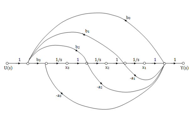
Fig 4: SFG for observable Form
Question: Find the observable canonical realization of the system H(s)=
Solution: The above transfer function can be also written as
H(s)=
Comparing above equation with standard equation we conclude that
The gains of forward paths are 
The feedback loop gains are 
The SFG satisfying above conditions will be

The observable canonical form can be obtained by converting the above SFG to block diagram
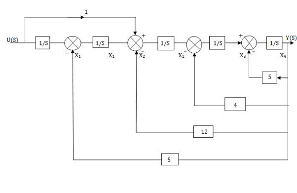
Fig 5. Observable canonical form can be obtained by converting the above SFG to block diagram
Controllable Canonical Form: In this the transfer function is divided into two parts as shown in below figure.
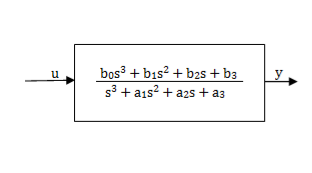
Fig 6: A third order system

Fig 7: Simplified representation of above system
G(s)= =
= 
 =
= ………..(7)
 =b0s3+b1s2+b2s+b3
The equation relating phase variable to input is given as

The equation relating output to phase variable can be given as(refer eq.(7))
y=b0 +b1
+b1 +b1
+b1 +b3x1
+b3x1
=b0(-a3x1-a2x2-a1x3+u)+b1x3+b2x2+b3x1
=(b3-a3b0)x1+(b2-a2b0)x2+(b1-a1b0)x3+b0u
The above equation in vector matrix form can be written as
y=[((b3-a3b0) (b2-a2b0) (b1-a1b0)] +b0u ……..(8)
The signal flow graph for above vector matrix equations is shown below
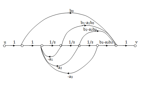
Fig 8: SFG for controllable form
Key takeaway
i) Matrix A is known as Bush form or companion form. Matrix B has all elements zero except the last element.
Ii) A system is observable if all its states can be determined by the output
Question: Find the controllable canonical realization of the following systems
a) H(s)=
b) H(s)=
Solution: a)H(s)=
Let H(s)=
 =
=
H1(s)= 1/s+6
1/s+6
X(s)=sX1(s)+6X1(s)
SX1(s)=X(s)+6X1(s)
We can get X1(s) by passing sX1(s) through integrator. The above equation can be realised as

Fig 9. H1(s)= 1/s+6
1/s+6
H2(s)= s+2
s+2
Similarly, Y(s)=sX1(s)+2X1(s)
H2(s)= s+2
s+2

Fig 10. H2(s)= s+2
s+2
The complete realization of transfer function can be obtained by combining the above two realizations. The complete realization will be

Fig 11. Complete realization of H(s)=
b)H(s)=
Let H(s)= =
= 
 =s+3
=s+3
Y(s)=sX1(s)+3X1(s)
The above transfer function can be realised as

Fig 12.  =s+3
=s+3
Now,  =
=
s2X1(s)=X(s)-2sX1(s)-5X1(s)
Assuming s2X1(s) is available the above transfer function can be realised as
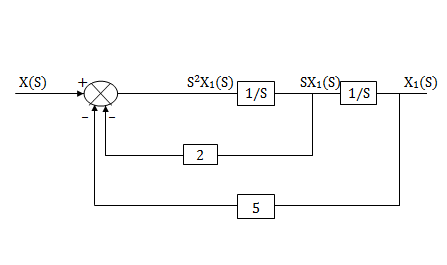
Fig 13.  =
=
The complete realization of transfer function can be obtained by combining the above two realizations. The complete realization will be
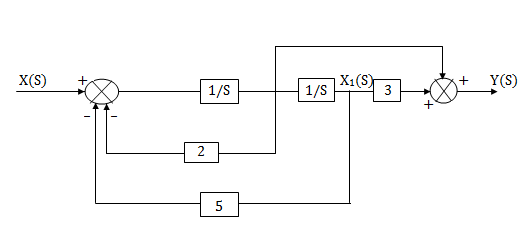
Fig 14. H(s)=
T= 
The overall transmittance Coverall gain can be determined by Masks formula.
Explanation
Pk forward path transmittance of k+n path from a specified i/p node to n o/p nods
While calculating ip node to n o/p nods.
While calculating ip no node should be encountered (used) more than ones.
 it is the graphics determined which involves of transmittances and multiple increases b/w non touching loops.
 = 1- [sum of all individual loop transmitting]
+[ sum of loop transmittance product of all possible non- touching loops]
-[sum of loop transmittance of all possible triples of non- touching loops]
 path factor associated with concered path & involves all a in the graphic which are isolated from forward path under consideration.
The path factor  for kthis equal to graph determinant of SFG which effect after erasing the kth path from the graph
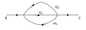
Q. Draw SFG for given block diagram?

Sol:

P1= G1 p2 =G2 Delta1 =1
L1= -G1 H1
 = 1-(-G1H1)
= 1+G1H1
T= G1+G2/1+G1H1
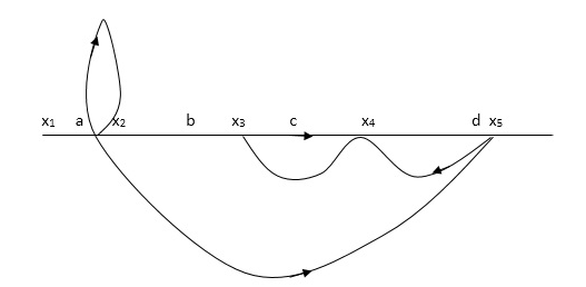
Q: Determine overall gain x5 and x1 Draw SFG
X2 = ax1+ f x2
X3= bx2 +exy
X4 = cx3+hx5
X5 =dx4 + gx2

P1 = abcd p2 = ag
L1 = f L2 = ce, L3= dh
 1 = 1
1 = 1
 2= 1-ce
 = 1-[L2+L2+L3] + [L1 L2 +L1 L3]
= 1-[f+ le = dh] + [fce +fdh]
T= abcd+ ag (1-ce)/1-[ftce + dh ] + (fce + fdh)
Key takeaway
- The function of individual element can be visualized from block diagram
- The signal travels along a branch in the direction of an arrow.
- The input signal is multiplied by the transmittance to obtain the o/p.
References:
1. I. J. Nagrath and M. Gopal, “Control Systems Engineering”, New Age International, 2009.
2. K. Ogata, “Modern Control Engineering”, Prentice Hall, 1991
3. M. Gopal, “Control Systems: Principles and Design”, McGraw Hill Education, 1997.
4. B. C. Kuo, “Automatic Control System”, Prentice Hall, 1995.


