Unit - 5
Frequency Domain analysis
The calculation of system parameters for higher order systems is difficult in time domain analysis. This can be overcome by frequency domain analysis. As the frequency response of a linear time invariant system is independent of amplitude and phase of the input test signal. The effect of noise and parameter variation in frequency domain can be easily computed.
In frequency response can be determine by calculating the phase and amplitude oof the given system transfer function. If a sinusoidal signal XG(j)sint then its amplitude will be
C(t) = XG(j)sint
= X|G(j)|  sint
sint
Magnitude = |G(j)|
Phase = G(j)
In polar form = |G(j)| 
Resonant Peak (Mr): The maximum value of magnitude is known as Resonant peak. The relative stability of the system can be determined by Mr. The larger the value of Mr the undesirable is the transient response.
Resonant Frequency (Wr): The frequency at which magnitude has maximum value.
Bandwidth: The band of frequencies lying between -3db points.
Cut-off frequency –The frequency at which the magnitude is 3db below its zero frequency.
Cut-off Rate – It is the slope of the log magnitude curve near the cut off frequency.


Fig 1 Frequency Domain Specification
The comparison of Mr and Mp is shown in figure. The two performance indices are correlated as both are functions of the damping factor ξ only. When subjected to step input the system with given value of Mr of its frequency response will exhibit a corresponding value of Mp.
Similarly the correlation of Wr and Wd is shown in figure for the given input step response [ from eqn(5) &eqn(8) ]
Wr/Wd = √(1- 2ξ2)/(1-ξ2)
Mp = Peak overshoot of step response
Mr = Resonant Peak of frequency response
Wr = Resonant frequency of Frequency response
Wd = Damping frequency of oscillation of step response.
From fig(1) it is clear that for ξ> 1/2, value of Mr does not exists.
Key takeaway
- Mr and Mpare correlated as both are functions of the damping factor ξ only
- When subjected to step input the system with given value of Mr of its frequency response will exhibit a corresponding value of Mp.
Bode Plot
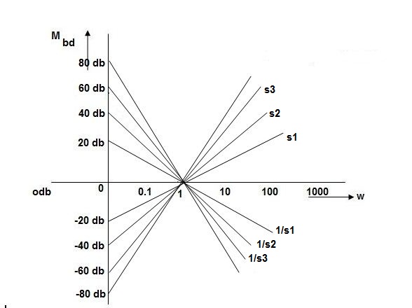
In polar plot any point gives the magnitude phase of the transfer function in bode we split magnitude and  plot.
plot.
Advantages
By looking at bode plot we can write the transfer function of system
Q. G(S) = 
Substitute S = j
G(j ) =
) = 
M = 
 = tan-1
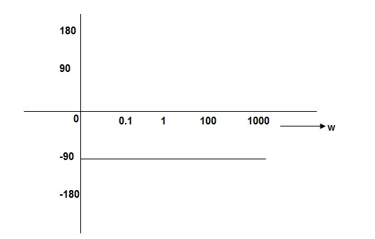
 = -900
Magnitude varies with ‘w’ but phase is constant.
MdB = +20 log10
MdB = -20 log10
Decade frequency:
W present = 10  past
past
Then  present is called decade frequency of
  past
past
 2 = 10
  1
1
 2 is decade frequency of
  1
1
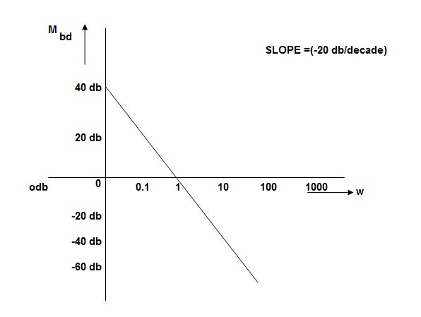
 MdB
MdB
0.0140
0.120
10 (shows pole at origin)
0-20
10-40
100-60
Slope = (20db/decade)

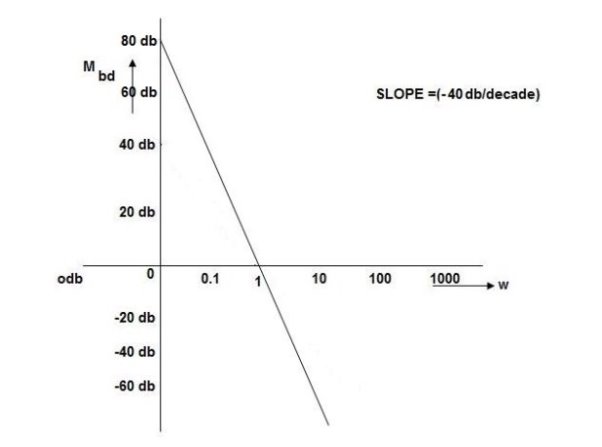
MAGNITUDE PLOT

PHASE PLOT
Q.G(S) = 
G(j ) =
) = 
M =  ;
;  = -1800 (-20tan-1
 )
)
MdB = +20 log  -2
-2
MdB = -40 log10
 MdB
MdB
0.0180
0.140
10(pole at origin)
10-40
100-80
Slope = 40dbdecade
Q. G(S) = S
M= W
 = 900
= 900
MdB = 20 log10
 MdB
MdB
0.01-40
0.1-20
10
1020
10090
100060
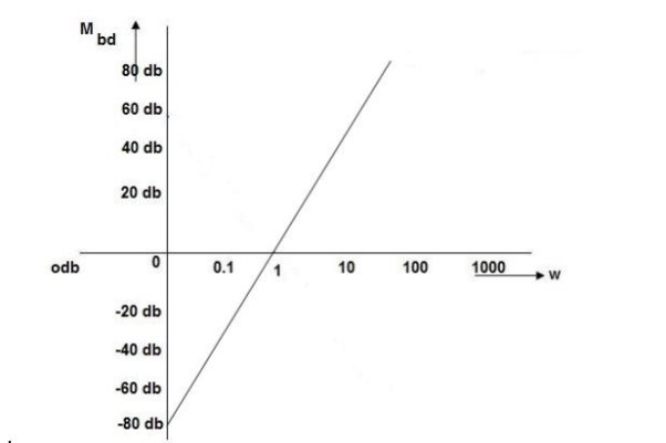
Q. G(S) = S2
M=  2MdB = 20 log10
 2
2
 = 1800 = 40 log10
WMdB
0.01-80
0.1-40
10
1040
10080

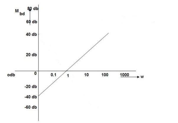
Q. (S) = 
G(j ) =
) = 
M = 
MdB = 20 log10 K-20 log10
 = tan-1(
 ) –tan-1(
 )
)
 = 0-900 = -900
K=1K=10  =-20 log10   0.014060 0.12040 1020 10-200 100-40-20 |

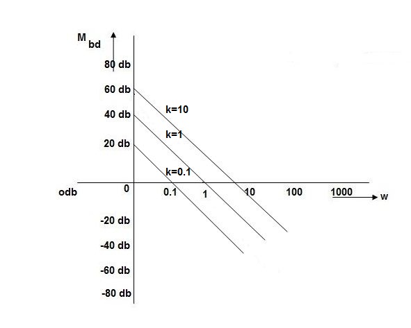
As we vary K  then plot shift by 20 log10K
i.e adding a d.c. To a.c. Quantity
Approximation of Bode Plot:
IF poles and zeros are not located at origin
G(S) = 
TF = 
M = 
MdB = -20 log10 (
 = -tan-1
Approximation:  T >> 1. So, we can neglect 1.
MdB = -20 log10
MdB = -20 log10 T . ;
T . ;  = -tan-1(
 T)
T)
Approximation:  T << 1. So, we can neglecting
 T.
T.
MdB= 0dB,  = 00
= 00
At a point both meet so equal i.e a time will come hence both approx become equal
-20 log10 T= 0
T= 0
 T= 1
T= 1
 corner frequency
At this frequency both the cases are equal
MdB = -20 log10
Now for 
MdB = -20 log10
= -20 log10
= -10 log102
MdB = 10
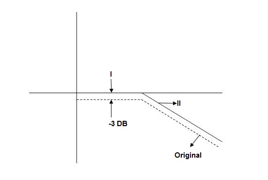
When we increase the value of  in app 2 and decrease the
  of app 1 so a RT comes when both cases are equal and hence for that value of
  where both app are equal gives max. Error we found above and is equal to 3dB
At corner frequency we have max error of -3dB
Que. G(S) = 
TF = 
M = 
MdB = -20 log10 ( at T=2
 MdB
MdB
1-20 log10
10-20 log10
100-20 log10
 MdB
MdB =
= =
= 
0.1-20 log10 = 1.73
  10-3
10-3
0.1-20 log10 = -0.1703
0.5-20 log10 = -3dB
1-20 log10 = -6.98
10-20 log10 = -26.03
100 -20 log10 = -46.02
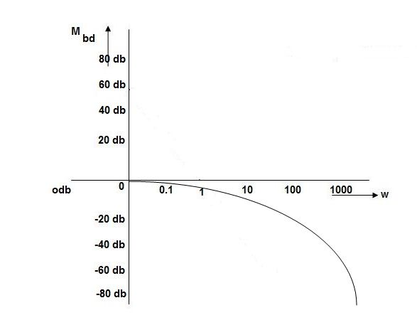
Fig 2. Magnitude Plot with approximation
Without approximation
For second order system
TF = 
TF = 
= 
= 
= 
M= 
MdB= 
Case 1 <<
<<
 << 1
<< 1
MdB= 20 log10 = 0 dB
Case 2  >>
>>
 >> 1
>> 1
MdB= -20 log10
= -20 log10
= -20 log10
 < 1
< 1  is very large so neglecting other two terms
MdB= -20 log10
= -40 log10
Case 3 . When case 1 is equal to case 2
-40 log10 = 0
= 0
 = 1
= 1

The natural frequency is our corner frequency
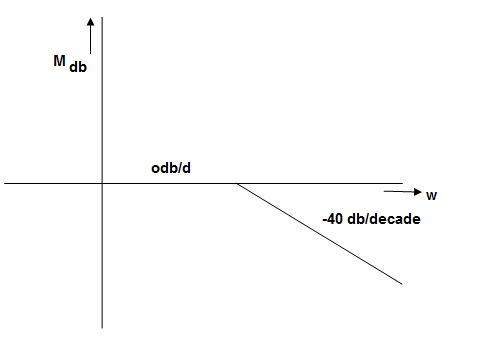
Fig 3. Magnitude Plot
Max error at  i.e at corner frequency
MdB= -20 log10
For 
MdB= -20 log10 
 error for
Completely the error depends upon the value of  (error at corner frequency)
The maximum error will be
MdB= -20 log10 
M = -20 log10 
 = 0
= 0

 is resonant frequency and at this frequency we are getting the maximum error so the magnitude will be
M = - +
+ 
= 
Mr =
MdB= -20 log10
MdB= -20 log10 
 = tan-1

Mr = 
Type of system | Initial slope | Intersection |
0 | 0 dB/decade | Parallel to 0 axis |
1 | -20 dB/decade | =K1 |
2 | -40 dB/decade | =K1/2 |
3 | -60 dB/decade | =K1/3 |
. | . | 1 |
. | . | 1 |
. | . | 1 |
N | -20N dB/decade | =K1/N |
Polar Plot
It gives the frequency response of the system. If the transfer function is given, then from the plot number of poles and zeros can be calculated.
Polar plot of some standard functions:
# TYPE ‘O’
Ex :1T(S) = 1/S + 1
(1). For polar plot substitute S=jw.
TF = 1/1 + jw
(2). Magnitude M = 1 + 0j / 1 + jw = 1/√1 + w2
(3). Phase φ = tan-1(0)/ tan-1w = - tan-1w
WMφ
0100
10.707 -450
∞0-900
The plot is shown in fig.

Fig 4. Polar Plot T(S) = 1/S + 1
Ex.2>. T(S) = 1/(S+1)(S+2)
(1). S = jw
TF = 1/(1+jw)(2+jw)
(2). M = 1/(1+jw)(2+jw) = 1/-w2 + 3jw + 2
M = 1/√1 + w2√4 + w2
(3). Φ = - tan-1 w - tan-1(w/2)
WMΦ
00.500
10.316 -71.560
20.158 -108.430
∞0-1800
The plot is shown in fig.

Fig 5. Polar Plot T(S) = 1/(S+1)(S+2)
Intersection of polar plot with imaginary axis will be when real part of Transfer function = 0
M = 1/(jw + 1)(jw + 2)
= 1/-w2 + j3w + 2
TYPE ‘1’
Ex.1 T(S) = 1/S
(1). S = jw
(2). M = 1/W
(3). Φ = -tan-1(W/O) = -900
WMφ
0∞-900
11-900
20.5-900
∞0-900
The plot is shown in fig.

Fig 6. Polar Plot T(S) = 1/S
Ex.2 T(S) = 1/S2
(1). S = jw
(2). M = 1/w2
(3). Φ = -tan-1(W/O)-tan-1(W/O) = -1800
WMΦ
0∞-1800
11-1800
20.25-1800
∞0-1800
The plot is shown in fig.

Fig 7. Polar Plot T(S) = 1/S2
Key takeaway
- For Polar Plot starting point depends upon type of system
- The terminating phase depends on order of the system.
TYPE 1 ORDER 2
Ex.1 T(S) = 1/S(S+1)
(1). M = 1/W√1+w2
(2). Φ = -900 - tan -1(W/T)
WMφ
0∞-900
10.707 -1350
20.45-153.40
∞0-1800
The plot is shown in fig.

Fig 8. Polar Plot T(S) = 1/S(S+1)
Ex.2TYPE 2 ORDER 3
T(s) = 1/S2(S+1)
(1). M = 1/w2√1+jw
(2). Φ = -1800 – tan-1W/T
The plot is shown in fig.

Fig 9. Polar Plot T(s) = 1/S2(S+1)
Bode Plot
Gain Cross Over Frequency
The frequency at which the bode plot culls the 0db axis is called as Gain Cross Over Frequency.

Fig 10. Gain cross over frequency
Phase Cross Over Frequency
The Frequency at which the phase plot culls the -1800 axis.

Fig 11. Phase Margin and Gain Margin
GM=MdB= -20 log [ G (jw)]
 .:
.: 
 .:
.: 
Key takeaway
i) More the difference b/WPC and WGC core are the stability of system
Ii) If GM is below 0dB axis than take +ve and stable. If GM above 0dB axis, that is take -ve
GM= ODB - 20 log M
Iii) The IM should also lie above -1800 for making the system (i.e. pm=+ve
Iv) For a stable system GM and PM should be -ve
v) GM and PM both should be +ve more the value of GM and PM more the system is stable.
Vi) If Wpc and Wgc are in same line Wpc= Wgc than system is marginally stable as we get GM=0dB.
Vii) When gain cross over frequency is smaller than phase curves over frequency the system is stable and vice versa.
Polar Plot
For open loop system number of poles o RHP are zero. So, the number of closed loop poles i.e zeros of Q(s) becomes
z=N+P
z=N
For open loop transfer function
G(s)H(s)= k/s(1+T1s)( 1+T2s)
The sinusoidal transfer function will be
G(jω)H(jω)=k/jω(1+ jωT1) (1+ jωT2)
The polar plot will be

Fig 12. Polar Plot for G(s)H(s)= k/s(1+T1s)( 1+T2s)
The intersection of polar plot with real axis can be obtained by equating imaginary part of G(jω)H(jω) to zero.
G(jω)H(jω) = -k[ω(T1+T2)+j(1- ω2T1T2)]/ ω(1+ ω2T12)( 1+ ω2T22)
The imaginary part is zero when
1-ω2T1T2 = 0
ωpc = 1/√ T1T2
At ωpc the magnitude of G(jω)H(jω) is
| G(jω)H(jω)| = -k T1T2/ T1+T2
The given system is stable when number of encirclements of -1+j0 is zero.

Fig 13. Finding GM of system from polar plot
Therefore, the condition for the system to be stable is k T1T2/ T1+T2<1.
When k < T1+T2/ T1T2 the point -1+j0 is not encircled by G(jω)H(jω) and system is stable. The gain is called critical gain kc= T1+T2/ T1T2.
For k<kc system is stable and when k=kc the plot passes through -1+j0 point which indicates the system has roots on jω-axis. For k>kc system is unstable as G(jω)H(jω) encircles the point -1+j0 once. There are two relative stability measurements which are
Gain Margin
From above figure we can say that at ω=ωpc the phase angle of  G(jω)H(jω) is 1800. The frequency at which the phase angle is 1800 is called as phase cross over frequency ωpc. Let A be magnitude at this frequency than if gain of the system is increased by 1/A the magnitude at ω=ωpc becomes 1 and hence G(jω)H(jω) locus passes through -1+j0 point and driving the system to the verse of instability. The gain margin can be defined as the reciprocal of the magnitude of open loop transfer function evaluated at the phase cross over frequency.
GM= 1/|G(jωpc)H(jωpc)|=1/A
 G(jω)H(jω) = - 1800
The GM in dB = -20logA.
Phase Margin
The frequency at which | G(jω)H(jω)|=1 is known as gain cross over frequency ωgc.As shown in figure bellow point A is the intersection of G(jω)H(jω)plot and the unit circle centred at the origin.
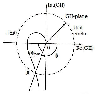
Fig 14. Finding PM of system from polar plot
Now draw a line connecting point A and origin and measure the phase angle between OA and positive real axis. The angle is known as phase angle of system at the gain cross over frequency.
 G(jωpc)H(jωpc)= ɸ
An additional phase lag ɸPM is introduced at this frequency then the phase angle  G(jωpc)H(jωpc) will become 1800 and the point A coincides with (-1+j0) driving the system to the verge of instability. This additional phase lag is known as phase margin. The value of phase margin can be obtained by
ɸPM= 1800 +  G(jω)H(jω) at ω=ωgc
ɸPM= 1800 + ɸ
Key takeaway
A zero GM in dB indicates critical stability. A positive GM indicates stability and a negative GM indicates instability.
For stable system PM is positive. A PM close to zero corresponds to highly oscillatory system.
Example
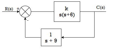
Q1) For the following system shown below find the phase margin and gain margin if the value of k=500by using Nyquist plot.

A1) G(s)H(s) = 500/s(s+6)(s+9)
The polar plot for above OLTF is shown in figure below.
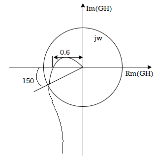
Fig 15. Polar Plot for given system
From figure we see A=0.6,
The GM in dB = -20logA.
= 4.43dB
PM = 1800-1650
= 150
Q2) For the system shown in figure, find the GM and PM using Nyquist plot for k=10. Find also range of k for stability?

A2) The transfer function is G(s) H(s) = 10(s+2(s+4)/s(s2 – 3s+10)
As the OLTF is unstable system so PM and GM concepts cannot be applied.
G(jω) H(jω) = 10(jω+2) (jω+4)/jω(-ω2 -3 jω+10)
| G(jω) H(jω)|= 10(√4+ω2)( √16+ω2)/ω√[(10-ω)2+9ω2]
 G(jω)H(jω) = -900 +tan-1(ω/2) + tan-1(ω/4) - tan-1 (-3ω/10- ω2)
The polar plot for above system is shown below.
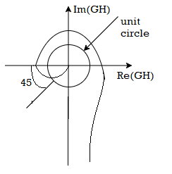
Fig 16. Polar plot for the given system
From figure we have A=2.6 and ɸ =-1350
The GM in dB = -20logA.
= -8.3dB
As GM is negative it indicates that system is open loop unstable.
PM = 1800-1650 = 450
The effect can be understood by plotting few bode plots as shown below
Q.1 Sketch the bode plot for transfer function
G(S) = 
- Replace S = j

G(j =
= 
This is type 0 system. So initial slope is 0 dB decade. The starting point is given as
20 log10 K = 20 log10 1000
= 60 dB
Corner frequency  1 =
1 =  = 10 rad/sec
 2 =
2 =  = 1000 rad/sec
Slope after  1 will be -20 dB/decade till second corner frequency i.e
 2 after
  2 the slope will be -40 dB/decade (-20+(-20)) as there are poles
2. For phase plot
 = tan-1 0.1
 - tan-1 0.001
For phase plot


100-900
200-9.450
300-104.80
400-110.360
500-115.420
600-120.00
700-124.170
800-127.940
900-131.350
1000 -134.420
The plot is shown in figure.

Fig 17. Magnitude Plot for G(S) = 
Q.2 For the given transfer function determine
G(S) = 
Gain cross over frequency phase cross over frequency phase mergence and gain margin
Initial slope = 1
N = 1, (K)1/N = 2
K = 2
Corner frequency
 1 =
1 =  = 2 (slope -20 dB/decade
 2 =
2 =  = 20 (slope -40 dB/decade

Phase
 = tan-1
 - tan-1 0.5
  - tan-1 0.05
 = 900- tan-1 0.5
  - tan-1 0.05


1-119.430
5-172.230
10-195.250
15-209.270
20-219.30
25-226.760
30-232.490
35-236.980
40-240.570
45-243.490
50-245.910
Finding  gc (gain cross over frequency
M = 
4 =  2 (
2 ( (
(
 6 (6.25
 104) + 0.252
 4 +
4 + 2 = 4
2 = 4
Let  2 = x
2 = x
X3 (6.25 104) + 0.252
 2 + x = 4
X1 = 2.46
X2 = -399.9
X3 = -6.50
For x1 = 2.46
 gc = 3.99 rad/sec(from plot )
For phase margin
PM = 1800 -
 = 900 – tan-1 (0.5×
 gc) – tan-1 (0.05 ×
  gc)
gc)
= -164.50
PM = 1800 - 164.50
= 15.50
For phase cross over frequency ( pc)
pc)
 = 900 – tan-1 (0.5
  ) – tan-1 (0.05
  )
)
-1800 = -900 – tan-1 (0.5  pc) – tan-1 (0.05
  pc)
pc)
-900 – tan-1 (0.5  pc) – tan-1 (0.05
  pc)
pc)
Taking than on both sides
Tan 900 = tan-1
Let tan-1 0.5  pc = A, tan-1 0.05
  pc = B
 = 00
= 00
 = 0
= 0
1 =0.5  pc 0.05
 pc
pc
 pc = 6.32 rad/sec
The plot is shown in figure.
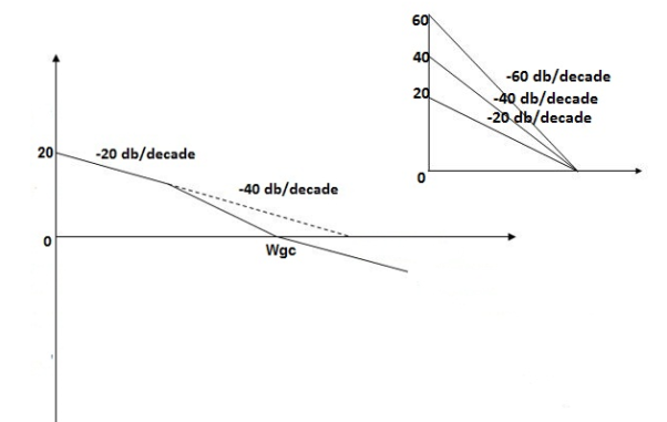
Fig 18. Magnitude Plot G(S) = 
Q3. For the given transfer function
G(S) = 
Plot the rode plot find PM and GM
T1 = 0.5  1 =
1 =  = 2 rad/sec
Zero so, slope (20 dB/decade)
T2 = 0.2  2 =
2 =  = 5 rad/sec
Pole, so slope (-20 dB/decade)
T3 = 0.1 = T4 = 0.1
 3 =
3 =  4 = 10 (2 pole) (-40 db/decade)
- Initial slope 0 dB/decade till
 1 = 2 rad/sec
 - From
 1 to
1 to 2 (i.e. 2 rad /sec to 5 rad/sec) slope will be 20 dB/decade
 - From
 2 to
2 to  3 the slope will be 0 dB/decade (20 + (-20))
 - From
 3,
3, 4 the slope will be -40 dB/decade (0-20-20)
Phase plot
 = tan-1 0.5
 - tan-1 0.2
 - tan-1 0.1
 - tan-1 0.1


500-177.30
1000-178.60
1500-179.10
2000-179.40
2500-179.50
3000-179.530
3500-179.60
GM = 00
PM = 61.460
The plot is shown in figure.


Fig 19. Magnitude and phase Plot for G(S) = 
Q4. For the given transfer function plot the bode plot (magnitude plot)
G(S) = 
Given transfer function
G(S) = 
Converting above transfer function to standard from
G(S) = 
= 
1. As type 1 system, so initial slope will be -20 dB/decade
2. Final slope will be -60 dB/decade as order of system decides the final slope
3. Corner frequency
T1 =  ,
,  11= 5 (zero)
T2 = 1,  2 = 1 (pole)
4. Initial slope will cut zero dB axis at
(K)1/N = 10
i.e = 10
= 10
5. Finding  n and
n and 
T(S) = 
T(S)= 
Comparing with standard second order system equation
S2+2 ns +
ns + n2
n2
 n = 11 rad/sec
 n = 5
n = 5
 11 = 5
 =
=  = 0.27
6. Maximum error
M = -20 log 2
= +6.5 dB
7. As K = 10, so whole plot will shift by 20 log 10 10 = 20 dB
The plot is shown in figure.

Fig 20. Magnitude Plot for G(S) = 
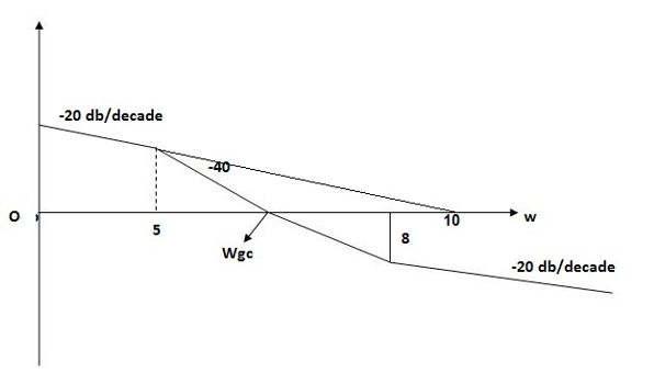
In this case we are given with a bode plot and we have to determine its transfer function. This can be best studied with the help of below given example.
Q. For the given plot determine the transfer function

From above figure we can conclude that
1. Initial slope = -20 dB/decade so type -1
2. Initial slope alls 0 dB axis at  = 10 so
K1/NN = 1
(K)1/N = 10.
3. Corner frequency
 1 =
1 =  = 0.2 rad/sec
 2 =
2 =  = 0.125 rad/sec
4. At  = 5 the slope becomes -40 dB/decade, so there is a pole at
  = 5 as slope changes from -20 dB/decade to -40 dB/decade
5. At  = 8 the slope changes from -40 dB/decade to -20 dB/decade hence is a zero at
  = 8 (-40+(+20)=20)
6. Hence transfer function is
T(S) = 
Transport lag is of nonminimum-phase behavior and has an excessive phase lag with no attenuation at high frequencies. Such transport lags normally exist in thermal, hydraulic, and pneumatic systems.

Consider the transport lag given by
G(j) = e-jT
The magnitude is always equal to unity since
|G(j)| = | cos T – j sin T| =1
Therefore, the log magnitude of the transport lag e-jωT is equal to 0 dB. The phase angle of the transport lag is
∠G(j) = - T (radians)
= - 57.3 T (degrees)
The phase angle varies linearly with the frequency ω. The phase-angle characteristic of transport lag is shown in Figure.
The order and relative degree of a system can be estimated from either the step response or the bode plot. The relative degree of a system is the difference between the order of the denominator over the order of the numerator of the transfer function and is the lowest order the system can be.
Step Response
If the response of the system to a non-zero step input has a zero slope when t = 0, the system must be second order or higher because the system has a relative degree of two or higher.
If the step response shows oscillations, the system must be a second order or higher underdamped system and have a relative degree of two or higher.
Bode Plot
The phase plot can be a good indicator of order. If the phase drops below -90 degrees, the system must be second order or higher. The relative degree of the system has to be at least as great as the number of multiples of -90 degrees achieved asymptotically at the lowest point on the phase plot of the system.
Identifying a System from the Step Response
DC Gain
The DC gain, K, is the ratio of the steady state step response to the magnitude of a step input.
Damping Ratio
For an underdamped second order system, the damping ratio can be calculated from the percent overshoot using the following formula:
 (1)
(1)
Where  is the maximum percent overshoot, which can be approximated from the plot of the step response.
Natural Frequency
The natural frequency of an underdamped second order system can be found from the damped natural frequency which can be measured off the plot of the step response and the damping ratio which was calculated above.
 (2)
(2)
Where,
(3)d = 2π/t
And t is the time interval between two consecutive peaks on the plot of the step response.
Identifying a System from the Bode Plot
DC Gain
The DC Gain of a system can be calculated from the magnitude of the bode plot when s = 0.
(4) K = 10M(0)/20
Where M(0) is the magnitude of the bode plot when j = 0.
Natural Frequency
The damping ratio of a system can be found with the DC Gain and the magnitude of the bode plot when the phase plot is -90 degrees.
(5) 
Identifying the System Parameters
If the type of system is known, then specific physical parameters may be found from the dynamic metrics determined above.
The general form of the transfer function of a first order system is
(6) G(s) = 
The general form of the transfer function of a second order system is
(7) G(s) = 
References:
1. Automatic Control Systems, Benjamin. C. Kuo, Prentice Hall of India, 7th Edition,1995.
2. Digital Control and State Variable Methods, M. Gopal, 2nd Edition, TMH, 2007.
3. Feedback and Control Systems, Stubberud, Schaum’s Outline Series, TataMcGraw-Hill, 2007.
4. Linear Control System Analysis and Design, John J. D’azzo & Constantine H.Houpis, Tata McGrow-Hill, Inc., 1995.
5. Modern Control Systems, Richard C. Dorf & Robert H. Bishop, Addison –Wesley, 1999.
Unit - 5
Frequency Domain analysis
The calculation of system parameters for higher order systems is difficult in time domain analysis. This can be overcome by frequency domain analysis. As the frequency response of a linear time invariant system is independent of amplitude and phase of the input test signal. The effect of noise and parameter variation in frequency domain can be easily computed.
In frequency response can be determine by calculating the phase and amplitude oof the given system transfer function. If a sinusoidal signal XG(j)sint then its amplitude will be
C(t) = XG(j)sint
= X|G(j)|  sint
sint
Magnitude = |G(j)|
Phase = G(j)
In polar form = |G(j)| 
Resonant Peak (Mr): The maximum value of magnitude is known as Resonant peak. The relative stability of the system can be determined by Mr. The larger the value of Mr the undesirable is the transient response.
Resonant Frequency (Wr): The frequency at which magnitude has maximum value.
Bandwidth: The band of frequencies lying between -3db points.
Cut-off frequency –The frequency at which the magnitude is 3db below its zero frequency.
Cut-off Rate – It is the slope of the log magnitude curve near the cut off frequency.

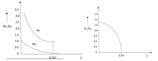
Fig 1 Frequency Domain Specification
The comparison of Mr and Mp is shown in figure. The two performance indices are correlated as both are functions of the damping factor ξ only. When subjected to step input the system with given value of Mr of its frequency response will exhibit a corresponding value of Mp.
Similarly the correlation of Wr and Wd is shown in figure for the given input step response [ from eqn(5) &eqn(8) ]
Wr/Wd = √(1- 2ξ2)/(1-ξ2)
Mp = Peak overshoot of step response
Mr = Resonant Peak of frequency response
Wr = Resonant frequency of Frequency response
Wd = Damping frequency of oscillation of step response.
From fig(1) it is clear that for ξ> 1/2, value of Mr does not exists.
Key takeaway
- Mr and Mpare correlated as both are functions of the damping factor ξ only
- When subjected to step input the system with given value of Mr of its frequency response will exhibit a corresponding value of Mp.
Bode Plot
In polar plot any point gives the magnitude phase of the transfer function in bode we split magnitude and  plot.
plot.
Advantages
By looking at bode plot we can write the transfer function of system
Q. G(S) = 
Substitute S = j
G(j ) =
) = 
M = 
 = tan-1
 = -900
Magnitude varies with ‘w’ but phase is constant.
MdB = +20 log10
MdB = -20 log10
Decade frequency:
W present = 10  past
past
Then  present is called decade frequency of
  past
past
 2 = 10
  1
1
 2 is decade frequency of
  1
1
 MdB
MdB
0.0140
0.120
10 (shows pole at origin)
0-20
10-40
100-60
Slope = (20db/decade)

MAGNITUDE PLOT

PHASE PLOT
Q.G(S) = 
G(j ) =
) = 
M =  ;
;  = -1800 (-20tan-1
 )
)
MdB = +20 log  -2
-2
MdB = -40 log10
 MdB
MdB
0.0180
0.140
10(pole at origin)
10-40
100-80
Slope = 40dbdecade
Q. G(S) = S
M= W
 = 900
= 900
MdB = 20 log10
 MdB
MdB
0.01-40
0.1-20
10
1020
10090
100060

Q. G(S) = S2
M=  2MdB = 20 log10
 2
2
 = 1800 = 40 log10
WMdB
0.01-80
0.1-40
10
1040
10080

Q. (S) = 
G(j ) =
) = 
M = 
MdB = 20 log10 K-20 log10
 = tan-1(
 ) –tan-1(
 )
)
 = 0-900 = -900
K=1K=10  =-20 log10   0.014060 0.12040 1020 10-200 100-40-20 |


As we vary K  then plot shift by 20 log10K
i.e adding a d.c. To a.c. Quantity
Approximation of Bode Plot:
IF poles and zeros are not located at origin
G(S) = 
TF = 
M = 
MdB = -20 log10 (
 = -tan-1
Approximation:  T >> 1. So, we can neglect 1.
MdB = -20 log10
MdB = -20 log10 T . ;
T . ;  = -tan-1(
 T)
T)
Approximation:  T << 1. So, we can neglecting
 T.
T.
MdB= 0dB,  = 00
= 00
At a point both meet so equal i.e a time will come hence both approx become equal
-20 log10 T= 0
T= 0
 T= 1
T= 1
 corner frequency
At this frequency both the cases are equal
MdB = -20 log10
Now for 
MdB = -20 log10
= -20 log10
= -10 log102
MdB = 10

When we increase the value of  in app 2 and decrease the
  of app 1 so a RT comes when both cases are equal and hence for that value of
  where both app are equal gives max. Error we found above and is equal to 3dB
At corner frequency we have max error of -3dB
Que. G(S) = 
TF = 
M = 
MdB = -20 log10 ( at T=2
 MdB
MdB
1-20 log10
10-20 log10
100-20 log10
 MdB
MdB =
= =
= 
0.1-20 log10 = 1.73
  10-3
10-3
0.1-20 log10 = -0.1703
0.5-20 log10 = -3dB
1-20 log10 = -6.98
10-20 log10 = -26.03
100 -20 log10 = -46.02

Fig 2. Magnitude Plot with approximation
Without approximation
For second order system
TF = 
TF = 
= 
= 
= 
M= 
MdB= 
Case 1 <<
<<
 << 1
<< 1
MdB= 20 log10 = 0 dB
Case 2  >>
>>
 >> 1
>> 1
MdB= -20 log10
= -20 log10
= -20 log10
 < 1
< 1  is very large so neglecting other two terms
MdB= -20 log10
= -40 log10
Case 3 . When case 1 is equal to case 2
-40 log10 = 0
= 0
 = 1
= 1

The natural frequency is our corner frequency

Fig 3. Magnitude Plot
Max error at  i.e at corner frequency
MdB= -20 log10
For 
MdB= -20 log10 
 error for
Completely the error depends upon the value of  (error at corner frequency)
The maximum error will be
MdB= -20 log10 
M = -20 log10 
 = 0
= 0

 is resonant frequency and at this frequency we are getting the maximum error so the magnitude will be
M = - +
+ 
= 
Mr =
MdB= -20 log10
MdB= -20 log10 
 = tan-1

Mr = 
Type of system | Initial slope | Intersection |
0 | 0 dB/decade | Parallel to 0 axis |
1 | -20 dB/decade | =K1 |
2 | -40 dB/decade | =K1/2 |
3 | -60 dB/decade | =K1/3 |
. | . | 1 |
. | . | 1 |
. | . | 1 |
N | -20N dB/decade | =K1/N |
Polar Plot
It gives the frequency response of the system. If the transfer function is given, then from the plot number of poles and zeros can be calculated.
Polar plot of some standard functions:
# TYPE ‘O’
Ex :1T(S) = 1/S + 1
(1). For polar plot substitute S=jw.
TF = 1/1 + jw
(2). Magnitude M = 1 + 0j / 1 + jw = 1/√1 + w2
(3). Phase φ = tan-1(0)/ tan-1w = - tan-1w
WMφ
0100
10.707 -450
∞0-900
The plot is shown in fig.

Fig 4. Polar Plot T(S) = 1/S + 1
Ex.2>. T(S) = 1/(S+1)(S+2)
(1). S = jw
TF = 1/(1+jw)(2+jw)
(2). M = 1/(1+jw)(2+jw) = 1/-w2 + 3jw + 2
M = 1/√1 + w2√4 + w2
(3). Φ = - tan-1 w - tan-1(w/2)
WMΦ
00.500
10.316 -71.560
20.158 -108.430
∞0-1800
The plot is shown in fig.

Fig 5. Polar Plot T(S) = 1/(S+1)(S+2)
Intersection of polar plot with imaginary axis will be when real part of Transfer function = 0
M = 1/(jw + 1)(jw + 2)
= 1/-w2 + j3w + 2
TYPE ‘1’
Ex.1 T(S) = 1/S
(1). S = jw
(2). M = 1/W
(3). Φ = -tan-1(W/O) = -900
WMφ
0∞-900
11-900
20.5-900
∞0-900
The plot is shown in fig.
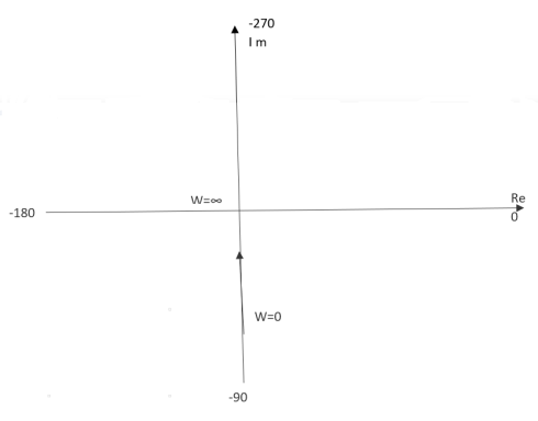
Fig 6. Polar Plot T(S) = 1/S
Ex.2 T(S) = 1/S2
(1). S = jw
(2). M = 1/w2
(3). Φ = -tan-1(W/O)-tan-1(W/O) = -1800
WMΦ
0∞-1800
11-1800
20.25-1800
∞0-1800
The plot is shown in fig.
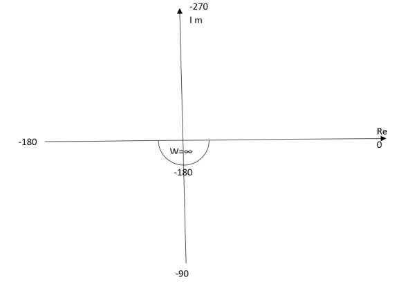
Fig 7. Polar Plot T(S) = 1/S2
Key takeaway
- For Polar Plot starting point depends upon type of system
- The terminating phase depends on order of the system.
TYPE 1 ORDER 2
Ex.1 T(S) = 1/S(S+1)
(1). M = 1/W√1+w2
(2). Φ = -900 - tan -1(W/T)
WMφ
0∞-900
10.707 -1350
20.45-153.40
∞0-1800
The plot is shown in fig.

Fig 8. Polar Plot T(S) = 1/S(S+1)
Ex.2TYPE 2 ORDER 3
T(s) = 1/S2(S+1)
(1). M = 1/w2√1+jw
(2). Φ = -1800 – tan-1W/T
The plot is shown in fig.
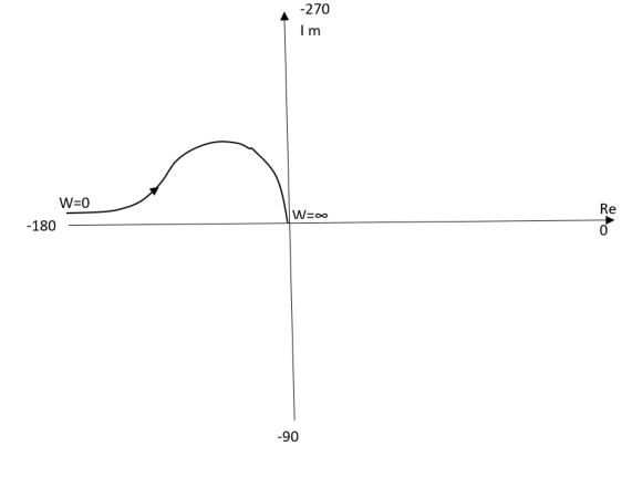
Fig 9. Polar Plot T(s) = 1/S2(S+1)
Bode Plot
Gain Cross Over Frequency
The frequency at which the bode plot culls the 0db axis is called as Gain Cross Over Frequency.

Fig 10. Gain cross over frequency
Phase Cross Over Frequency
The Frequency at which the phase plot culls the -1800 axis.

Fig 11. Phase Margin and Gain Margin
GM=MdB= -20 log [ G (jw)]
 .:
.: 
 .:
.: 
Key takeaway
i) More the difference b/WPC and WGC core are the stability of system
Ii) If GM is below 0dB axis than take +ve and stable. If GM above 0dB axis, that is take -ve
GM= ODB - 20 log M
Iii) The IM should also lie above -1800 for making the system (i.e. pm=+ve
Iv) For a stable system GM and PM should be -ve
v) GM and PM both should be +ve more the value of GM and PM more the system is stable.
Vi) If Wpc and Wgc are in same line Wpc= Wgc than system is marginally stable as we get GM=0dB.
Vii) When gain cross over frequency is smaller than phase curves over frequency the system is stable and vice versa.
Polar Plot
For open loop system number of poles o RHP are zero. So, the number of closed loop poles i.e zeros of Q(s) becomes
z=N+P
z=N
For open loop transfer function
G(s)H(s)= k/s(1+T1s)( 1+T2s)
The sinusoidal transfer function will be
G(jω)H(jω)=k/jω(1+ jωT1) (1+ jωT2)
The polar plot will be

Fig 12. Polar Plot for G(s)H(s)= k/s(1+T1s)( 1+T2s)
The intersection of polar plot with real axis can be obtained by equating imaginary part of G(jω)H(jω) to zero.
G(jω)H(jω) = -k[ω(T1+T2)+j(1- ω2T1T2)]/ ω(1+ ω2T12)( 1+ ω2T22)
The imaginary part is zero when
1-ω2T1T2 = 0
ωpc = 1/√ T1T2
At ωpc the magnitude of G(jω)H(jω) is
| G(jω)H(jω)| = -k T1T2/ T1+T2
The given system is stable when number of encirclements of -1+j0 is zero.
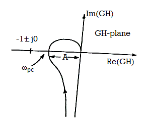
Fig 13. Finding GM of system from polar plot
Therefore, the condition for the system to be stable is k T1T2/ T1+T2<1.
When k < T1+T2/ T1T2 the point -1+j0 is not encircled by G(jω)H(jω) and system is stable. The gain is called critical gain kc= T1+T2/ T1T2.
For k<kc system is stable and when k=kc the plot passes through -1+j0 point which indicates the system has roots on jω-axis. For k>kc system is unstable as G(jω)H(jω) encircles the point -1+j0 once. There are two relative stability measurements which are
Gain Margin
From above figure we can say that at ω=ωpc the phase angle of  G(jω)H(jω) is 1800. The frequency at which the phase angle is 1800 is called as phase cross over frequency ωpc. Let A be magnitude at this frequency than if gain of the system is increased by 1/A the magnitude at ω=ωpc becomes 1 and hence G(jω)H(jω) locus passes through -1+j0 point and driving the system to the verse of instability. The gain margin can be defined as the reciprocal of the magnitude of open loop transfer function evaluated at the phase cross over frequency.
GM= 1/|G(jωpc)H(jωpc)|=1/A
 G(jω)H(jω) = - 1800
The GM in dB = -20logA.
Phase Margin
The frequency at which | G(jω)H(jω)|=1 is known as gain cross over frequency ωgc.As shown in figure bellow point A is the intersection of G(jω)H(jω)plot and the unit circle centred at the origin.

Fig 14. Finding PM of system from polar plot
Now draw a line connecting point A and origin and measure the phase angle between OA and positive real axis. The angle is known as phase angle of system at the gain cross over frequency.
 G(jωpc)H(jωpc)= ɸ
An additional phase lag ɸPM is introduced at this frequency then the phase angle  G(jωpc)H(jωpc) will become 1800 and the point A coincides with (-1+j0) driving the system to the verge of instability. This additional phase lag is known as phase margin. The value of phase margin can be obtained by
ɸPM= 1800 +  G(jω)H(jω) at ω=ωgc
ɸPM= 1800 + ɸ
Key takeaway
A zero GM in dB indicates critical stability. A positive GM indicates stability and a negative GM indicates instability.
For stable system PM is positive. A PM close to zero corresponds to highly oscillatory system.
Example
Q1) For the following system shown below find the phase margin and gain margin if the value of k=500by using Nyquist plot.

A1) G(s)H(s) = 500/s(s+6)(s+9)
The polar plot for above OLTF is shown in figure below.

Fig 15. Polar Plot for given system
From figure we see A=0.6,
The GM in dB = -20logA.
= 4.43dB
PM = 1800-1650
= 150
Q2) For the system shown in figure, find the GM and PM using Nyquist plot for k=10. Find also range of k for stability?
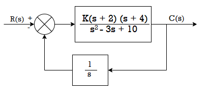
A2) The transfer function is G(s) H(s) = 10(s+2(s+4)/s(s2 – 3s+10)
As the OLTF is unstable system so PM and GM concepts cannot be applied.
G(jω) H(jω) = 10(jω+2) (jω+4)/jω(-ω2 -3 jω+10)
| G(jω) H(jω)|= 10(√4+ω2)( √16+ω2)/ω√[(10-ω)2+9ω2]
 G(jω)H(jω) = -900 +tan-1(ω/2) + tan-1(ω/4) - tan-1 (-3ω/10- ω2)
The polar plot for above system is shown below.

Fig 16. Polar plot for the given system
From figure we have A=2.6 and ɸ =-1350
The GM in dB = -20logA.
= -8.3dB
As GM is negative it indicates that system is open loop unstable.
PM = 1800-1650 = 450
The effect can be understood by plotting few bode plots as shown below
Q.1 Sketch the bode plot for transfer function
G(S) = 
- Replace S = j

G(j =
= 
This is type 0 system. So initial slope is 0 dB decade. The starting point is given as
20 log10 K = 20 log10 1000
= 60 dB
Corner frequency  1 =
1 =  = 10 rad/sec
 2 =
2 =  = 1000 rad/sec
Slope after  1 will be -20 dB/decade till second corner frequency i.e
 2 after
  2 the slope will be -40 dB/decade (-20+(-20)) as there are poles
2. For phase plot
 = tan-1 0.1
 - tan-1 0.001
For phase plot


100-900
200-9.450
300-104.80
400-110.360
500-115.420
600-120.00
700-124.170
800-127.940
900-131.350
1000 -134.420
The plot is shown in figure.
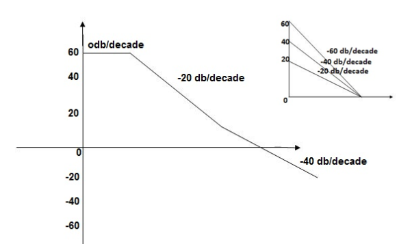
Fig 17. Magnitude Plot for G(S) = 
Q.2 For the given transfer function determine
G(S) = 
Gain cross over frequency phase cross over frequency phase mergence and gain margin
Initial slope = 1
N = 1, (K)1/N = 2
K = 2
Corner frequency
 1 =
1 =  = 2 (slope -20 dB/decade
 2 =
2 =  = 20 (slope -40 dB/decade

Phase
 = tan-1
 - tan-1 0.5
  - tan-1 0.05
 = 900- tan-1 0.5
  - tan-1 0.05


1-119.430
5-172.230
10-195.250
15-209.270
20-219.30
25-226.760
30-232.490
35-236.980
40-240.570
45-243.490
50-245.910
Finding  gc (gain cross over frequency
M = 
4 =  2 (
2 ( (
(
 6 (6.25
 104) + 0.252
 4 +
4 + 2 = 4
2 = 4
Let  2 = x
2 = x
X3 (6.25 104) + 0.252
 2 + x = 4
X1 = 2.46
X2 = -399.9
X3 = -6.50
For x1 = 2.46
 gc = 3.99 rad/sec(from plot )
For phase margin
PM = 1800 -
 = 900 – tan-1 (0.5×
 gc) – tan-1 (0.05 ×
  gc)
gc)
= -164.50
PM = 1800 - 164.50
= 15.50
For phase cross over frequency ( pc)
pc)
 = 900 – tan-1 (0.5
  ) – tan-1 (0.05
  )
)
-1800 = -900 – tan-1 (0.5  pc) – tan-1 (0.05
  pc)
pc)
-900 – tan-1 (0.5  pc) – tan-1 (0.05
  pc)
pc)
Taking than on both sides
Tan 900 = tan-1
Let tan-1 0.5  pc = A, tan-1 0.05
  pc = B
 = 00
= 00
 = 0
= 0
1 =0.5  pc 0.05
 pc
pc
 pc = 6.32 rad/sec
The plot is shown in figure.

Fig 18. Magnitude Plot G(S) = 
Q3. For the given transfer function
G(S) = 
Plot the rode plot find PM and GM
T1 = 0.5  1 =
1 =  = 2 rad/sec
Zero so, slope (20 dB/decade)
T2 = 0.2  2 =
2 =  = 5 rad/sec
Pole, so slope (-20 dB/decade)
T3 = 0.1 = T4 = 0.1
 3 =
3 =  4 = 10 (2 pole) (-40 db/decade)
- Initial slope 0 dB/decade till
 1 = 2 rad/sec
 - From
 1 to
1 to 2 (i.e. 2 rad /sec to 5 rad/sec) slope will be 20 dB/decade
 - From
 2 to
2 to  3 the slope will be 0 dB/decade (20 + (-20))
 - From
 3,
3, 4 the slope will be -40 dB/decade (0-20-20)
Phase plot
 = tan-1 0.5
 - tan-1 0.2
 - tan-1 0.1
 - tan-1 0.1


500-177.30
1000-178.60
1500-179.10
2000-179.40
2500-179.50
3000-179.530
3500-179.60
GM = 00
PM = 61.460
The plot is shown in figure.
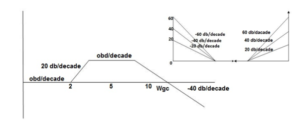

Fig 19. Magnitude and phase Plot for G(S) = 
Q4. For the given transfer function plot the bode plot (magnitude plot)
G(S) = 
Given transfer function
G(S) = 
Converting above transfer function to standard from
G(S) = 
= 
1. As type 1 system, so initial slope will be -20 dB/decade
2. Final slope will be -60 dB/decade as order of system decides the final slope
3. Corner frequency
T1 =  ,
,  11= 5 (zero)
T2 = 1,  2 = 1 (pole)
4. Initial slope will cut zero dB axis at
(K)1/N = 10
i.e = 10
= 10
5. Finding  n and
n and 
T(S) = 
T(S)= 
Comparing with standard second order system equation
S2+2 ns +
ns + n2
n2
 n = 11 rad/sec
 n = 5
n = 5
 11 = 5
 =
=  = 0.27
6. Maximum error
M = -20 log 2
= +6.5 dB
7. As K = 10, so whole plot will shift by 20 log 10 10 = 20 dB
The plot is shown in figure.
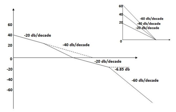
Fig 20. Magnitude Plot for G(S) = 
In this case we are given with a bode plot and we have to determine its transfer function. This can be best studied with the help of below given example.
Q. For the given plot determine the transfer function
From above figure we can conclude that
1. Initial slope = -20 dB/decade so type -1
2. Initial slope alls 0 dB axis at  = 10 so
K1/NN = 1
(K)1/N = 10.
3. Corner frequency
 1 =
1 =  = 0.2 rad/sec
 2 =
2 =  = 0.125 rad/sec
4. At  = 5 the slope becomes -40 dB/decade, so there is a pole at
  = 5 as slope changes from -20 dB/decade to -40 dB/decade
5. At  = 8 the slope changes from -40 dB/decade to -20 dB/decade hence is a zero at
  = 8 (-40+(+20)=20)
6. Hence transfer function is
T(S) = 
Transport lag is of nonminimum-phase behavior and has an excessive phase lag with no attenuation at high frequencies. Such transport lags normally exist in thermal, hydraulic, and pneumatic systems.

Consider the transport lag given by
G(j) = e-jT
The magnitude is always equal to unity since
|G(j)| = | cos T – j sin T| =1
Therefore, the log magnitude of the transport lag e-jωT is equal to 0 dB. The phase angle of the transport lag is
∠G(j) = - T (radians)
= - 57.3 T (degrees)
The phase angle varies linearly with the frequency ω. The phase-angle characteristic of transport lag is shown in Figure.
The order and relative degree of a system can be estimated from either the step response or the bode plot. The relative degree of a system is the difference between the order of the denominator over the order of the numerator of the transfer function and is the lowest order the system can be.
Step Response
If the response of the system to a non-zero step input has a zero slope when t = 0, the system must be second order or higher because the system has a relative degree of two or higher.
If the step response shows oscillations, the system must be a second order or higher underdamped system and have a relative degree of two or higher.
Bode Plot
The phase plot can be a good indicator of order. If the phase drops below -90 degrees, the system must be second order or higher. The relative degree of the system has to be at least as great as the number of multiples of -90 degrees achieved asymptotically at the lowest point on the phase plot of the system.
Identifying a System from the Step Response
DC Gain
The DC gain, K, is the ratio of the steady state step response to the magnitude of a step input.
Damping Ratio
For an underdamped second order system, the damping ratio can be calculated from the percent overshoot using the following formula:
 (1)
(1)
Where  is the maximum percent overshoot, which can be approximated from the plot of the step response.
Natural Frequency
The natural frequency of an underdamped second order system can be found from the damped natural frequency which can be measured off the plot of the step response and the damping ratio which was calculated above.
 (2)
(2)
Where,
(3)d = 2π/t
And t is the time interval between two consecutive peaks on the plot of the step response.
Identifying a System from the Bode Plot
DC Gain
The DC Gain of a system can be calculated from the magnitude of the bode plot when s = 0.
(4) K = 10M(0)/20
Where M(0) is the magnitude of the bode plot when j = 0.
Natural Frequency
The damping ratio of a system can be found with the DC Gain and the magnitude of the bode plot when the phase plot is -90 degrees.
(5) 
Identifying the System Parameters
If the type of system is known, then specific physical parameters may be found from the dynamic metrics determined above.
The general form of the transfer function of a first order system is
(6) G(s) = 
The general form of the transfer function of a second order system is
(7) G(s) = 
References:
1. Automatic Control Systems, Benjamin. C. Kuo, Prentice Hall of India, 7th Edition,1995.
2. Digital Control and State Variable Methods, M. Gopal, 2nd Edition, TMH, 2007.
3. Feedback and Control Systems, Stubberud, Schaum’s Outline Series, TataMcGraw-Hill, 2007.
4. Linear Control System Analysis and Design, John J. D’azzo & Constantine H.Houpis, Tata McGrow-Hill, Inc., 1995.
5. Modern Control Systems, Richard C. Dorf & Robert H. Bishop, Addison –Wesley, 1999.
Unit - 5
Frequency Domain analysis
The calculation of system parameters for higher order systems is difficult in time domain analysis. This can be overcome by frequency domain analysis. As the frequency response of a linear time invariant system is independent of amplitude and phase of the input test signal. The effect of noise and parameter variation in frequency domain can be easily computed.
In frequency response can be determine by calculating the phase and amplitude oof the given system transfer function. If a sinusoidal signal XG(j)sint then its amplitude will be
C(t) = XG(j)sint
= X|G(j)|  sint
sint
Magnitude = |G(j)|
Phase = G(j)
In polar form = |G(j)| 
Resonant Peak (Mr): The maximum value of magnitude is known as Resonant peak. The relative stability of the system can be determined by Mr. The larger the value of Mr the undesirable is the transient response.
Resonant Frequency (Wr): The frequency at which magnitude has maximum value.
Bandwidth: The band of frequencies lying between -3db points.
Cut-off frequency –The frequency at which the magnitude is 3db below its zero frequency.
Cut-off Rate – It is the slope of the log magnitude curve near the cut off frequency.
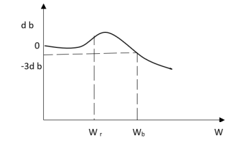

Fig 1 Frequency Domain Specification
The comparison of Mr and Mp is shown in figure. The two performance indices are correlated as both are functions of the damping factor ξ only. When subjected to step input the system with given value of Mr of its frequency response will exhibit a corresponding value of Mp.
Similarly the correlation of Wr and Wd is shown in figure for the given input step response [ from eqn(5) &eqn(8) ]
Wr/Wd = √(1- 2ξ2)/(1-ξ2)
Mp = Peak overshoot of step response
Mr = Resonant Peak of frequency response
Wr = Resonant frequency of Frequency response
Wd = Damping frequency of oscillation of step response.
From fig(1) it is clear that for ξ> 1/2, value of Mr does not exists.
Key takeaway
- Mr and Mpare correlated as both are functions of the damping factor ξ only
- When subjected to step input the system with given value of Mr of its frequency response will exhibit a corresponding value of Mp.
Bode Plot
In polar plot any point gives the magnitude phase of the transfer function in bode we split magnitude and  plot.
plot.
Advantages
By looking at bode plot we can write the transfer function of system
Q. G(S) = 
Substitute S = j
G(j ) =
) = 
M = 
 = tan-1
 = -900
Magnitude varies with ‘w’ but phase is constant.
MdB = +20 log10
MdB = -20 log10
Decade frequency:
W present = 10  past
past
Then  present is called decade frequency of
  past
past
 2 = 10
  1
1
 2 is decade frequency of
  1
1
 MdB
MdB
0.0140
0.120
10 (shows pole at origin)
0-20
10-40
100-60
Slope = (20db/decade)
MAGNITUDE PLOT
PHASE PLOT
Q.G(S) = 
G(j ) =
) = 
M =  ;
;  = -1800 (-20tan-1
 )
)
MdB = +20 log  -2
-2
MdB = -40 log10
 MdB
MdB
0.0180
0.140
10(pole at origin)
10-40
100-80
Slope = 40dbdecade
Q. G(S) = S
M= W
 = 900
= 900
MdB = 20 log10
 MdB
MdB
0.01-40
0.1-20
10
1020
10090
100060

Q. G(S) = S2
M=  2MdB = 20 log10
 2
2
 = 1800 = 40 log10
WMdB
0.01-80
0.1-40
10
1040
10080
Q. (S) = 
G(j ) =
) = 
M = 
MdB = 20 log10 K-20 log10
 = tan-1(
 ) –tan-1(
 )
)
 = 0-900 = -900
K=1K=10  =-20 log10   0.014060 0.12040 1020 10-200 100-40-20 |


As we vary K  then plot shift by 20 log10K
i.e adding a d.c. To a.c. Quantity
Approximation of Bode Plot:
IF poles and zeros are not located at origin
G(S) = 
TF = 
M = 
MdB = -20 log10 (
 = -tan-1
Approximation:  T >> 1. So, we can neglect 1.
MdB = -20 log10
MdB = -20 log10 T . ;
T . ;  = -tan-1(
 T)
T)
Approximation:  T << 1. So, we can neglecting
 T.
T.
MdB= 0dB,  = 00
= 00
At a point both meet so equal i.e a time will come hence both approx become equal
-20 log10 T= 0
T= 0
 T= 1
T= 1
 corner frequency
At this frequency both the cases are equal
MdB = -20 log10
Now for 
MdB = -20 log10
= -20 log10
= -10 log102
MdB = 10

When we increase the value of  in app 2 and decrease the
  of app 1 so a RT comes when both cases are equal and hence for that value of
  where both app are equal gives max. Error we found above and is equal to 3dB
At corner frequency we have max error of -3dB
Que. G(S) = 
TF = 
M = 
MdB = -20 log10 ( at T=2
 MdB
MdB
1-20 log10
10-20 log10
100-20 log10
 MdB
MdB =
= =
= 
0.1-20 log10 = 1.73
  10-3
10-3
0.1-20 log10 = -0.1703
0.5-20 log10 = -3dB
1-20 log10 = -6.98
10-20 log10 = -26.03
100 -20 log10 = -46.02

Fig 2. Magnitude Plot with approximation
Without approximation
For second order system
TF = 
TF = 
= 
= 
= 
M= 
MdB= 
Case 1 <<
<<
 << 1
<< 1
MdB= 20 log10 = 0 dB
Case 2  >>
>>
 >> 1
>> 1
MdB= -20 log10
= -20 log10
= -20 log10
 < 1
< 1  is very large so neglecting other two terms
MdB= -20 log10
= -40 log10
Case 3 . When case 1 is equal to case 2
-40 log10 = 0
= 0
 = 1
= 1

The natural frequency is our corner frequency

Fig 3. Magnitude Plot
Max error at  i.e at corner frequency
MdB= -20 log10
For 
MdB= -20 log10 
 error for
Completely the error depends upon the value of  (error at corner frequency)
The maximum error will be
MdB= -20 log10 
M = -20 log10 
 = 0
= 0

 is resonant frequency and at this frequency we are getting the maximum error so the magnitude will be
M = - +
+ 
= 
Mr =
MdB= -20 log10
MdB= -20 log10 
 = tan-1

Mr = 
Type of system | Initial slope | Intersection |
0 | 0 dB/decade | Parallel to 0 axis |
1 | -20 dB/decade | =K1 |
2 | -40 dB/decade | =K1/2 |
3 | -60 dB/decade | =K1/3 |
. | . | 1 |
. | . | 1 |
. | . | 1 |
N | -20N dB/decade | =K1/N |
Polar Plot
It gives the frequency response of the system. If the transfer function is given, then from the plot number of poles and zeros can be calculated.
Polar plot of some standard functions:
# TYPE ‘O’
Ex :1T(S) = 1/S + 1
(1). For polar plot substitute S=jw.
TF = 1/1 + jw
(2). Magnitude M = 1 + 0j / 1 + jw = 1/√1 + w2
(3). Phase φ = tan-1(0)/ tan-1w = - tan-1w
WMφ
0100
10.707 -450
∞0-900
The plot is shown in fig.
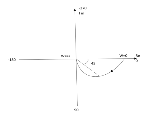
Fig 4. Polar Plot T(S) = 1/S + 1
Ex.2>. T(S) = 1/(S+1)(S+2)
(1). S = jw
TF = 1/(1+jw)(2+jw)
(2). M = 1/(1+jw)(2+jw) = 1/-w2 + 3jw + 2
M = 1/√1 + w2√4 + w2
(3). Φ = - tan-1 w - tan-1(w/2)
WMΦ
00.500
10.316 -71.560
20.158 -108.430
∞0-1800
The plot is shown in fig.
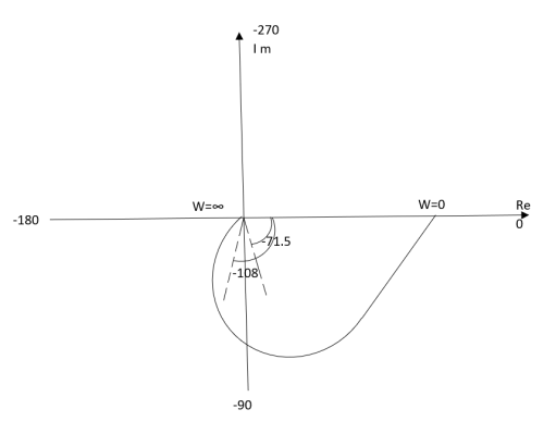
Fig 5. Polar Plot T(S) = 1/(S+1)(S+2)
Intersection of polar plot with imaginary axis will be when real part of Transfer function = 0
M = 1/(jw + 1)(jw + 2)
= 1/-w2 + j3w + 2
TYPE ‘1’
Ex.1 T(S) = 1/S
(1). S = jw
(2). M = 1/W
(3). Φ = -tan-1(W/O) = -900
WMφ
0∞-900
11-900
20.5-900
∞0-900
The plot is shown in fig.

Fig 6. Polar Plot T(S) = 1/S
Ex.2 T(S) = 1/S2
(1). S = jw
(2). M = 1/w2
(3). Φ = -tan-1(W/O)-tan-1(W/O) = -1800
WMΦ
0∞-1800
11-1800
20.25-1800
∞0-1800
The plot is shown in fig.

Fig 7. Polar Plot T(S) = 1/S2
Key takeaway
- For Polar Plot starting point depends upon type of system
- The terminating phase depends on order of the system.
TYPE 1 ORDER 2
Ex.1 T(S) = 1/S(S+1)
(1). M = 1/W√1+w2
(2). Φ = -900 - tan -1(W/T)
WMφ
0∞-900
10.707 -1350
20.45-153.40
∞0-1800
The plot is shown in fig.
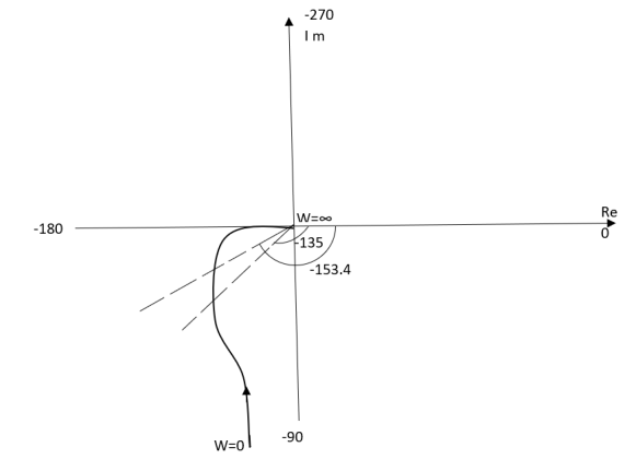
Fig 8. Polar Plot T(S) = 1/S(S+1)
Ex.2TYPE 2 ORDER 3
T(s) = 1/S2(S+1)
(1). M = 1/w2√1+jw
(2). Φ = -1800 – tan-1W/T
The plot is shown in fig.

Fig 9. Polar Plot T(s) = 1/S2(S+1)
Bode Plot
Gain Cross Over Frequency
The frequency at which the bode plot culls the 0db axis is called as Gain Cross Over Frequency.
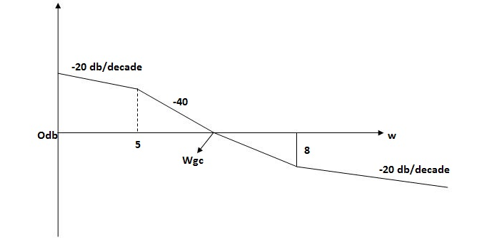
Fig 10. Gain cross over frequency
Phase Cross Over Frequency
The Frequency at which the phase plot culls the -1800 axis.
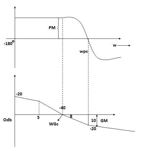
Fig 11. Phase Margin and Gain Margin
GM=MdB= -20 log [ G (jw)]
 .:
.: 
 .:
.: 
Key takeaway
i) More the difference b/WPC and WGC core are the stability of system
Ii) If GM is below 0dB axis than take +ve and stable. If GM above 0dB axis, that is take -ve
GM= ODB - 20 log M
Iii) The IM should also lie above -1800 for making the system (i.e. pm=+ve
Iv) For a stable system GM and PM should be -ve
v) GM and PM both should be +ve more the value of GM and PM more the system is stable.
Vi) If Wpc and Wgc are in same line Wpc= Wgc than system is marginally stable as we get GM=0dB.
Vii) When gain cross over frequency is smaller than phase curves over frequency the system is stable and vice versa.
Polar Plot
For open loop system number of poles o RHP are zero. So, the number of closed loop poles i.e zeros of Q(s) becomes
z=N+P
z=N
For open loop transfer function
G(s)H(s)= k/s(1+T1s)( 1+T2s)
The sinusoidal transfer function will be
G(jω)H(jω)=k/jω(1+ jωT1) (1+ jωT2)
The polar plot will be
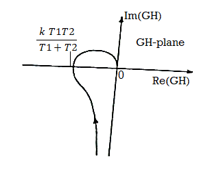
Fig 12. Polar Plot for G(s)H(s)= k/s(1+T1s)( 1+T2s)
The intersection of polar plot with real axis can be obtained by equating imaginary part of G(jω)H(jω) to zero.
G(jω)H(jω) = -k[ω(T1+T2)+j(1- ω2T1T2)]/ ω(1+ ω2T12)( 1+ ω2T22)
The imaginary part is zero when
1-ω2T1T2 = 0
ωpc = 1/√ T1T2
At ωpc the magnitude of G(jω)H(jω) is
| G(jω)H(jω)| = -k T1T2/ T1+T2
The given system is stable when number of encirclements of -1+j0 is zero.

Fig 13. Finding GM of system from polar plot
Therefore, the condition for the system to be stable is k T1T2/ T1+T2<1.
When k < T1+T2/ T1T2 the point -1+j0 is not encircled by G(jω)H(jω) and system is stable. The gain is called critical gain kc= T1+T2/ T1T2.
For k<kc system is stable and when k=kc the plot passes through -1+j0 point which indicates the system has roots on jω-axis. For k>kc system is unstable as G(jω)H(jω) encircles the point -1+j0 once. There are two relative stability measurements which are
Gain Margin
From above figure we can say that at ω=ωpc the phase angle of  G(jω)H(jω) is 1800. The frequency at which the phase angle is 1800 is called as phase cross over frequency ωpc. Let A be magnitude at this frequency than if gain of the system is increased by 1/A the magnitude at ω=ωpc becomes 1 and hence G(jω)H(jω) locus passes through -1+j0 point and driving the system to the verse of instability. The gain margin can be defined as the reciprocal of the magnitude of open loop transfer function evaluated at the phase cross over frequency.
GM= 1/|G(jωpc)H(jωpc)|=1/A
 G(jω)H(jω) = - 1800
The GM in dB = -20logA.
Phase Margin
The frequency at which | G(jω)H(jω)|=1 is known as gain cross over frequency ωgc.As shown in figure bellow point A is the intersection of G(jω)H(jω)plot and the unit circle centred at the origin.

Fig 14. Finding PM of system from polar plot
Now draw a line connecting point A and origin and measure the phase angle between OA and positive real axis. The angle is known as phase angle of system at the gain cross over frequency.
 G(jωpc)H(jωpc)= ɸ
An additional phase lag ɸPM is introduced at this frequency then the phase angle  G(jωpc)H(jωpc) will become 1800 and the point A coincides with (-1+j0) driving the system to the verge of instability. This additional phase lag is known as phase margin. The value of phase margin can be obtained by
ɸPM= 1800 +  G(jω)H(jω) at ω=ωgc
ɸPM= 1800 + ɸ
Key takeaway
A zero GM in dB indicates critical stability. A positive GM indicates stability and a negative GM indicates instability.
For stable system PM is positive. A PM close to zero corresponds to highly oscillatory system.
Example
Q1) For the following system shown below find the phase margin and gain margin if the value of k=500by using Nyquist plot.
A1) G(s)H(s) = 500/s(s+6)(s+9)
The polar plot for above OLTF is shown in figure below.

Fig 15. Polar Plot for given system
From figure we see A=0.6,
The GM in dB = -20logA.
= 4.43dB
PM = 1800-1650
= 150
Q2) For the system shown in figure, find the GM and PM using Nyquist plot for k=10. Find also range of k for stability?

A2) The transfer function is G(s) H(s) = 10(s+2(s+4)/s(s2 – 3s+10)
As the OLTF is unstable system so PM and GM concepts cannot be applied.
G(jω) H(jω) = 10(jω+2) (jω+4)/jω(-ω2 -3 jω+10)
| G(jω) H(jω)|= 10(√4+ω2)( √16+ω2)/ω√[(10-ω)2+9ω2]
 G(jω)H(jω) = -900 +tan-1(ω/2) + tan-1(ω/4) - tan-1 (-3ω/10- ω2)
The polar plot for above system is shown below.

Fig 16. Polar plot for the given system
From figure we have A=2.6 and ɸ =-1350
The GM in dB = -20logA.
= -8.3dB
As GM is negative it indicates that system is open loop unstable.
PM = 1800-1650 = 450
The effect can be understood by plotting few bode plots as shown below
Q.1 Sketch the bode plot for transfer function
G(S) = 
- Replace S = j

G(j =
= 
This is type 0 system. So initial slope is 0 dB decade. The starting point is given as
20 log10 K = 20 log10 1000
= 60 dB
Corner frequency  1 =
1 =  = 10 rad/sec
 2 =
2 =  = 1000 rad/sec
Slope after  1 will be -20 dB/decade till second corner frequency i.e
 2 after
  2 the slope will be -40 dB/decade (-20+(-20)) as there are poles
2. For phase plot
 = tan-1 0.1
 - tan-1 0.001
For phase plot


100-900
200-9.450
300-104.80
400-110.360
500-115.420
600-120.00
700-124.170
800-127.940
900-131.350
1000 -134.420
The plot is shown in figure.

Fig 17. Magnitude Plot for G(S) = 
Q.2 For the given transfer function determine
G(S) = 
Gain cross over frequency phase cross over frequency phase mergence and gain margin
Initial slope = 1
N = 1, (K)1/N = 2
K = 2
Corner frequency
 1 =
1 =  = 2 (slope -20 dB/decade
 2 =
2 =  = 20 (slope -40 dB/decade

Phase
 = tan-1
 - tan-1 0.5
  - tan-1 0.05
 = 900- tan-1 0.5
  - tan-1 0.05


1-119.430
5-172.230
10-195.250
15-209.270
20-219.30
25-226.760
30-232.490
35-236.980
40-240.570
45-243.490
50-245.910
Finding  gc (gain cross over frequency
M = 
4 =  2 (
2 ( (
(
 6 (6.25
 104) + 0.252
 4 +
4 + 2 = 4
2 = 4
Let  2 = x
2 = x
X3 (6.25 104) + 0.252
 2 + x = 4
X1 = 2.46
X2 = -399.9
X3 = -6.50
For x1 = 2.46
 gc = 3.99 rad/sec(from plot )
For phase margin
PM = 1800 -
 = 900 – tan-1 (0.5×
 gc) – tan-1 (0.05 ×
  gc)
gc)
= -164.50
PM = 1800 - 164.50
= 15.50
For phase cross over frequency ( pc)
pc)
 = 900 – tan-1 (0.5
  ) – tan-1 (0.05
  )
)
-1800 = -900 – tan-1 (0.5  pc) – tan-1 (0.05
  pc)
pc)
-900 – tan-1 (0.5  pc) – tan-1 (0.05
  pc)
pc)
Taking than on both sides
Tan 900 = tan-1
Let tan-1 0.5  pc = A, tan-1 0.05
  pc = B
 = 00
= 00
 = 0
= 0
1 =0.5  pc 0.05
 pc
pc
 pc = 6.32 rad/sec
The plot is shown in figure.

Fig 18. Magnitude Plot G(S) = 
Q3. For the given transfer function
G(S) = 
Plot the rode plot find PM and GM
T1 = 0.5  1 =
1 =  = 2 rad/sec
Zero so, slope (20 dB/decade)
T2 = 0.2  2 =
2 =  = 5 rad/sec
Pole, so slope (-20 dB/decade)
T3 = 0.1 = T4 = 0.1
 3 =
3 =  4 = 10 (2 pole) (-40 db/decade)
- Initial slope 0 dB/decade till
 1 = 2 rad/sec
 - From
 1 to
1 to 2 (i.e. 2 rad /sec to 5 rad/sec) slope will be 20 dB/decade
 - From
 2 to
2 to  3 the slope will be 0 dB/decade (20 + (-20))
 - From
 3,
3, 4 the slope will be -40 dB/decade (0-20-20)
Phase plot
 = tan-1 0.5
 - tan-1 0.2
 - tan-1 0.1
 - tan-1 0.1


500-177.30
1000-178.60
1500-179.10
2000-179.40
2500-179.50
3000-179.530
3500-179.60
GM = 00
PM = 61.460
The plot is shown in figure.

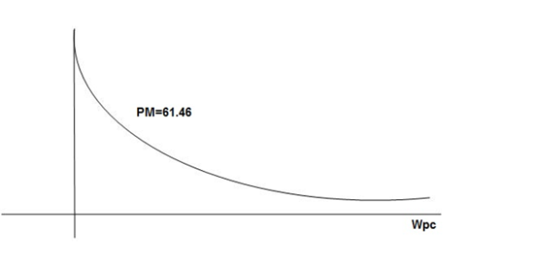
Fig 19. Magnitude and phase Plot for G(S) = 
Q4. For the given transfer function plot the bode plot (magnitude plot)
G(S) = 
Given transfer function
G(S) = 
Converting above transfer function to standard from
G(S) = 
= 
1. As type 1 system, so initial slope will be -20 dB/decade
2. Final slope will be -60 dB/decade as order of system decides the final slope
3. Corner frequency
T1 =  ,
,  11= 5 (zero)
T2 = 1,  2 = 1 (pole)
4. Initial slope will cut zero dB axis at
(K)1/N = 10
i.e = 10
= 10
5. Finding  n and
n and 
T(S) = 
T(S)= 
Comparing with standard second order system equation
S2+2 ns +
ns + n2
n2
 n = 11 rad/sec
 n = 5
n = 5
 11 = 5
 =
=  = 0.27
6. Maximum error
M = -20 log 2
= +6.5 dB
7. As K = 10, so whole plot will shift by 20 log 10 10 = 20 dB
The plot is shown in figure.

Fig 20. Magnitude Plot for G(S) = 
In this case we are given with a bode plot and we have to determine its transfer function. This can be best studied with the help of below given example.
Q. For the given plot determine the transfer function

From above figure we can conclude that
1. Initial slope = -20 dB/decade so type -1
2. Initial slope alls 0 dB axis at  = 10 so
K1/NN = 1
(K)1/N = 10.
3. Corner frequency
 1 =
1 =  = 0.2 rad/sec
 2 =
2 =  = 0.125 rad/sec
4. At  = 5 the slope becomes -40 dB/decade, so there is a pole at
  = 5 as slope changes from -20 dB/decade to -40 dB/decade
5. At  = 8 the slope changes from -40 dB/decade to -20 dB/decade hence is a zero at
  = 8 (-40+(+20)=20)
6. Hence transfer function is
T(S) = 
Transport lag is of nonminimum-phase behavior and has an excessive phase lag with no attenuation at high frequencies. Such transport lags normally exist in thermal, hydraulic, and pneumatic systems.
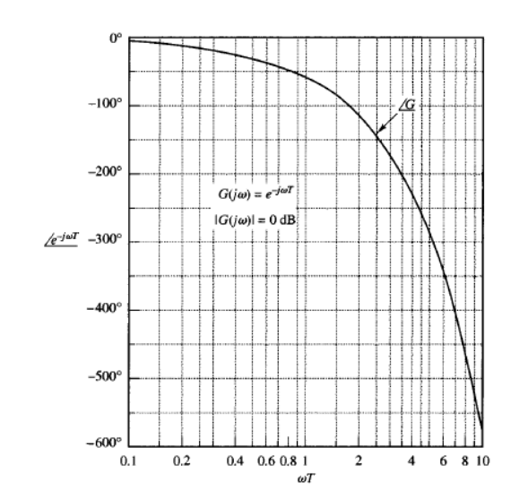
Consider the transport lag given by
G(j) = e-jT
The magnitude is always equal to unity since
|G(j)| = | cos T – j sin T| =1
Therefore, the log magnitude of the transport lag e-jωT is equal to 0 dB. The phase angle of the transport lag is
∠G(j) = - T (radians)
= - 57.3 T (degrees)
The phase angle varies linearly with the frequency ω. The phase-angle characteristic of transport lag is shown in Figure.
The order and relative degree of a system can be estimated from either the step response or the bode plot. The relative degree of a system is the difference between the order of the denominator over the order of the numerator of the transfer function and is the lowest order the system can be.
Step Response
If the response of the system to a non-zero step input has a zero slope when t = 0, the system must be second order or higher because the system has a relative degree of two or higher.
If the step response shows oscillations, the system must be a second order or higher underdamped system and have a relative degree of two or higher.
Bode Plot
The phase plot can be a good indicator of order. If the phase drops below -90 degrees, the system must be second order or higher. The relative degree of the system has to be at least as great as the number of multiples of -90 degrees achieved asymptotically at the lowest point on the phase plot of the system.
Identifying a System from the Step Response
DC Gain
The DC gain, K, is the ratio of the steady state step response to the magnitude of a step input.
Damping Ratio
For an underdamped second order system, the damping ratio can be calculated from the percent overshoot using the following formula:
 (1)
(1)
Where  is the maximum percent overshoot, which can be approximated from the plot of the step response.
Natural Frequency
The natural frequency of an underdamped second order system can be found from the damped natural frequency which can be measured off the plot of the step response and the damping ratio which was calculated above.
 (2)
(2)
Where,
(3)d = 2π/t
And t is the time interval between two consecutive peaks on the plot of the step response.
Identifying a System from the Bode Plot
DC Gain
The DC Gain of a system can be calculated from the magnitude of the bode plot when s = 0.
(4) K = 10M(0)/20
Where M(0) is the magnitude of the bode plot when j = 0.
Natural Frequency
The damping ratio of a system can be found with the DC Gain and the magnitude of the bode plot when the phase plot is -90 degrees.
(5) 
Identifying the System Parameters
If the type of system is known, then specific physical parameters may be found from the dynamic metrics determined above.
The general form of the transfer function of a first order system is
(6) G(s) = 
The general form of the transfer function of a second order system is
(7) G(s) = 
References:
1. Automatic Control Systems, Benjamin. C. Kuo, Prentice Hall of India, 7th Edition,1995.
2. Digital Control and State Variable Methods, M. Gopal, 2nd Edition, TMH, 2007.
3. Feedback and Control Systems, Stubberud, Schaum’s Outline Series, TataMcGraw-Hill, 2007.
4. Linear Control System Analysis and Design, John J. D’azzo & Constantine H.Houpis, Tata McGrow-Hill, Inc., 1995.
5. Modern Control Systems, Richard C. Dorf & Robert H. Bishop, Addison –Wesley, 1999.