Unit - 6
State space representation of Continuous Time systems
The state of a system is a minimal set of variables known as state variables. The knowledge of these variables at any instance of time together with the knowledge of the inputs for the same instance of time determines the complete behaviour of the system. The fewer drawbacks in the transfer function method for representing any system led to the use of state variables in the analysis of the system. Few advantages are listed below:
- The state-space can be used for linear or nonlinear, time-variant, or time-invariant systems.
- It is easier to apply where Laplace transform cannot be applied.
- The nth order differential equation can be expressed as the 'n' equation of the first order.
- It is a time-domain method.
- As this is a time-domain method, therefore this method is suitable for digital computer computation.
- Based on the given performance index, this system can be designed for optimal conditions.
Representation of state-space: The system shown below has ‘m’ inputs, ‘p, outputs, and ‘n’ number of state variables. The state equation gives us the relation between the state variables and the inputs.

Fig 1 State variable
So, the above system shown can be described through equations as
 =f1 (x1, x2,…….xn , u1, u2……… ,um)
 = f2 (x1, x2,…….xn , u1, u2……… ,um)
 =f1 (x1, x2,…….xn , u1, u2……… ,um) (1)
The above set of equations can be represented as
 =f(x(t),u(t)) (2)
As we are concerned for time invariant system, for which the term  in (1) is a linear combination of state variables and input. So,
 (t)=2tx1+x2+u1+u2 (3)
 =a11x1(t)+a12x2(t)+…a1nxn(t)+b11u1(t)+b12u2(t)+…….+b1mum(t)
 =a21x1(t)+a22x2(t)+…a2nxn(t)+b21u1(t)+b22u2(t)+…….+b2mum(t)
 =an1x1(t)+an2x2(t)+…annxn(t)+bn1u1(t)+bn2u2(t)+…….+bnmum(t)
The above equation can be represented in matrix form as given below
 (4)
(4)
The above coefficients aij and bji in equation (4) can be written in a vector-matrix form as
 =Ax(t)+Bu(t) (5)
Key takeaway
The state of a system is a minimal set of variables known as state variables.
The vector-matrix form is given as  =Ax(t)+Bu(t)
Calculation of transfer function from state model:
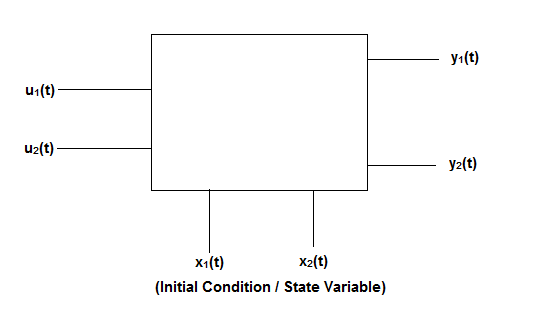
Fig 2: State model
The above figure shows the state model of a system with two inputs u1(t) and u2(t), and having outputs y1(t) and y2(t). As discussed in above section 4.1, we know that the output equation is given as
Y(t)=Cx(t)+Du(t) (9)
 (10)
(10)
Taking L.T of equation (9)
Y(s)=CX(s)+DU(s) (11)
Taking L.T of equation (10)
SX(s)=AX(s)+BU(s) (12)
X(s)=[SI-A]-1BU(s) (13)
Y(s)=CX(s)+DU(s)
Y(s)=C{[SI-A]-1BU(s)} + DU(s)
 = C{[SI-A]-1B} + D (14)
[SI-A]-1=
The denominator of equation (14) is the characteristic equation
[SI-A]=0
State space representation for electrical and mechanical system
Physical variable form: The state variables selected here are the physical quantities of the system, which can be measured. The selection of these variables can be directly related to the physical system because the solution of state equation is related to the time variation of the system variables.
The number of energy storing elements in any system is equal to the number of state variables. Below shown are few electrical circuits, just to brush up the concept of energy storing elements and state variable relation.

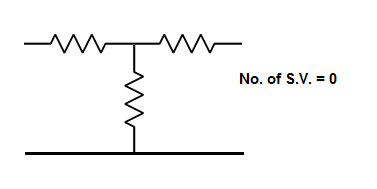
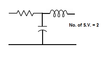
Now calculating the state equation and output equation for state variable analysis.
State Equation and Output equation:
Number of output=Number of output equation

Fig 3. State Model
Considering multiple input and multiple output system, with two inputs u1(t)and u2(t), and two outputs y1(t) and y2(t) respectively.
y1(t)=c11x1(t)+c12x2(t)+d11u1(t)+d12u2(t)
y2(t)=c21x1(t)+c22x2(t)+d21u1(t)+d22u2(t)

The output equation is given as
Y(t)=CX(t)+DU(t)


# Now finding State Equation
Number of energy-storing elements= Number of state variables

=a11x1(t)+a12x2(t)+b11u1(t)+b12u2(t)

=a21x1(t)+a22x2(t)+b21u1(t)+b22u2(t)

The state equation is then given as
 =Ax(t)+Bu(t)
Key takeaway
The number of energy storing element= Number of state variables
We should always take voltage across the inductor L, and current through capacitor C.
Question: Obtain the state space representation for the given electrical system
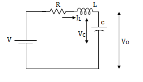
Solution: The state model is given as
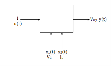
The state model shows that there are two energy storing elements L, C. As we already know that Number of state variables is equal to the number of energy storing elements.Hence we have two state variables[x1(t) and x2(t)]. We have one output V0(taken across the capacitor) and input u(t).
The output equation is then given as
Y(t)=CX(t)+DU(t)
V0=Vc= x1(t) ….(a)
Hence output equation becomes
V0= x1(t)
y(t)=[1 0]  +[0]u(t)
So, C=[1 0] D=[0]
Now writing the state equation
 =Ax(t)+Bu(t)
For that applying KVL in the above circuit
V=ILR+L +Vc
+Vc
State Equation is  =Ax(t)+Bu(t)
 =
=
x1(t)=Vc
 =
=
IL=C
 =
=
 =
= =
=
 =(1/C) x2(t) ……….(b)
 =
= =
=
VL=L
 =
= =VL/L
=VL/L
From KVL
L =VL=V-ILR-VC
 =
= =
=
 =
= …………….(c)
From equation (b) and (c)
 = [0 1/c]
  + [0 0]u(t)
 =[-1/L -R/L]
  + [1/L 0]
Now writing the state equation
 =Ax(t)+Bu(t)

Hence


Question: Obtatin the state space representation for the given electircal system
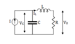
Solution: The state model shows that there are two energy storing elements L, C. As we already know that Number of state variables is equal to the number of energy storing elements.Hence we have two state variables[x1(t) and x2(t)]. We have one output V0(taken across capacitor) and input u(t).
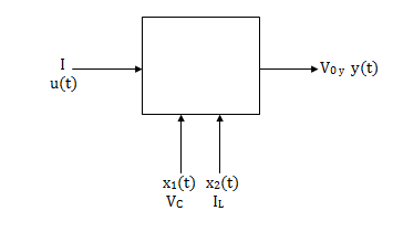
Here output is V0. But from above electrical circuit V0=ILR
V0=x2(t)R
y(t)=V0= [0 R] + [0] u(t)
The output equation is given as
Y(t)=CX(t)+DU(t)
C=[0 R] D=[0]
Now finding state equation,we apply KCL in the given electrical circuit
I=IC+IL
 =
=
But I-IL=IC
 =
=
 =
=
 =
=
 =
= x2(t)+
 ……..(a)
 =[0 1/C]
 + [1/C 0]
 …….(b)
 =
= =
=
Applying KVL in the given electrical circuit we get
VC=VL+ILR
VC-ILR=VL=L

 =
=
 =[1/L -R/L]
  + [0] u(t) ………….(c)
From equation (b) and (c) we have
Now writing the state equation
 =Ax(t)+Bu(t)
 =
= +
+ 
Hence A= B=
B= 
Note:We should always take voltage across the inductor L, and current through capacitor C.
Mechanical form: In this type of systems the potential and kinetic energy of a mass are function of position and velocity of the mass respectively. Hence, the velocity and position are selected as state variables.
Question: Write the state equation for the mechanical system shown below?
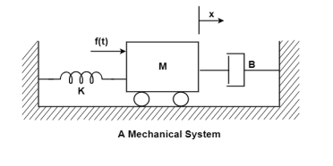
The free body diagram is

The position and velocity are state variables hence,
x1(t)=x(t)
x2(t)=
 =
= =x2(t)
 =
=
The system equation will be

 =
=
 =
=
 =
=
The state equations are
 = x2(t)
 =
=
 =
= +
+ f(t)
f(t)
The phase variables are defined as the state variables obtained from any one of the system variables and its derivatives. The nth order linear differential equation for given input y(t) and output u(t) is given as
y(n)+a1y(n-1)+………..+an-1 +any=bou(m)+……+bm-1
 + bm u. ….. (15)
The initial conditions are expressed as y(0), ,…..,y(n-1)(0).
The transfer function assuming all initial conditions zero is
T(s)= =[b0sm+b1sm-1+….+bm-1s+bm/[sn+a1sn-1+……..+an-1s+an] ……(16)
Considering simple case when there are no zeros in the system, the transfer function becomes
T(s)= =[b]/ [sn+a1sn-1+……..+an-1s+an] …….(17)
For above transfer function the differential equation is given as
y(n)+a1y(n-1)+………..+an-1 +any=bu …….(18)
Let x1=y
x2=
…….
xn=y(n-1)
From (18) the differential equation is given as


……….

 =-anx1-an-1x2-…….-a1xn+bu
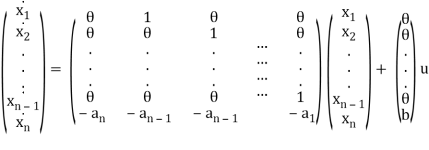
 =Ax+Bu ……….(19)
Note: Matrix A is known as Bush form or companion form. Matrix B has all elements zero except the last element.
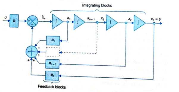
The output equation is given as y=x1
y=Cx ……….(20)
Where C =[1 0 0………..0]
The phase variable formation for the transfer function can be obtained by the below mentioned two canonical forms.
Controllability: A control system is said to be completely controllable if it’s possible to transfer the state of system from initial state to any other required state.
[S]= [B AB AB2 AB3 ------------------- An-1B]
Kalman’s Test: A system is said to be completely controllable if determinant of matrix is not equal to zero, or the rank of the following matrix should be to ‘n’.
n---- order of the matrix.
If  ≠0 then completely controllable
If  =0 then not controllable
Question: A system is represented by following state model A=  B=
B= find whether it is controllable or not?
Solution: A=  B=
B=
So order of matrix is n=2
[S]=[B AB]
= 
 =0 hence, system is not controllable.
Observability: A system is said to be completely observable if it is possible to determine the initial state of system by observing the output for finite interval of time.
Calman’s Test: A system is said to be completely observable within the determinant of following matrix is not equal to zero, or, the matrix rank should be equal to 1.
[Q]= [CT ATCT (AT)2CT ----------(AT)n-1CT]
If ≠0 then completely observable
=0 then not observable
Question: A system is represented by following state model A=  B=
B= , C=[1 1] test whether the system is observable or not?
Solution: AT=  CT=
CT=
[Q]=[CT ATCT]
=
=
=
=0
 =0 hence not observable.
Just as with continuous-time control, we can choose to utilize a transfer function approach or a state variable approach to control. In this chapter we will utilize the transfer function approach, while in the remainder of these notes we will utilize the state variable approach. In this brief chapter we first discuss implementing discrete-time transfer functions, then talk about some common conventions used in control system.
Just as in continuous-time we will represent signals in either the time domain or the transform domain, which in this case is the z-transform domain. A simple input-output transfer function block is shown in Figure. While in the continuous time-domain it might be somewhat difficult to solve for the output in terms of the input in the time-domain, in the discrete-time domain we can just use the recursive relationship from the transfer function. Specifically, if we have the transfer function G(z), then we can write it as

Where n ≥ m. Converting this to the time domain, the output y(k) can be written in terms of previous output values and the current and previous input values as
y(k) = −a1y(k − 1) − a2y(k − 2) + ···− any(k − n) + b0u(k) + b1u(k − 1) + ... + bmu(k − m)
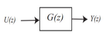
Fig 4. Discrete-time transfer function
This is an Infinite Impulse Response (IIR) filter, since the output at any time depends on both previous outputs and previous inputs. If the output depended only on previous inputs, it would be a Finite Impulse Response (FIR) filter.
State Equations of Sampled Data Systems
Let us assume that the following continuous time system is subject to sampling process with an interval of T
 =Ax(t) + Bu(t)
The above equation is the state equation
y(t) = Cx(t) +Du(t)
The above equation is the output equation.
We know that the solution to above state equation is
x(t) = ( t – t0) x(t0) + 
Since the inputs are constants in between two sampling instants, one can write:
u(τ) = u(kT) for, kT ≤ τ ≤ (k + 1) T
Which implies that the following expression is valid within the interval kT ≤ τ≤ (k + 1)T if we consider t0 = kT
x(t) = ( t – kT) x(kT) + 
Let us denote
 by θ(t – KT)
Then we can write
x(t) = (t – kT)x(kT) + θ(t – Kt)u(kT)
If t = (k + 1)T,
x((k + 1)T) = (T)x(kT) + θ(T)u(kT)
Where
(T) = eAT and θ(T) = 
If t ′ = τ−kT, we can rewrite θ(T) as
θ(T) = 
If we consider φ(T) = A¯ and θ(T) = B¯. Similarly, by setting t = kT, one can show that the output equation also has a similar form as that of the continuous time one.
When T = 1,
x(k + 1) = (1)x(k) + θ(1) u(k)
y(k) = Cx(k) + Du(k)
State Equations of Inherently Discrete Systems
When a discrete system is composed of all digital signals, the state and output equations can be described by
x(k + 1) = Ax(k) + Bu(k)
y(k) = Cx(k) + Du(k)
Discrete Time Approximation of Continuous Time State Space Model
Let us consider the dynamical system described by the state space mode. By approximating the derivative at t = kT using forward difference, we can write:


And
y(kT) = Cx(kT) + Du(kT)
x((k + 1)T) = (I + TA)x(kT) + TBu(kT)
If T=1
x(k + 1) = (I + A) x(k) + Bu(k)
y(k) = C x (k) + Du(k)
We can thus conclude from the discussions so far that the discrete time state variable model of a system can be described by
x(k + 1) = Ax(k) + Bu(k)
y(k) = Cx(k) + Du(k)
Where A, B are either the descriptions of an all-digital system or obtained by sampling the continuous time process.
Stability is the most important issue in control system design. Before discussing the stability test let us first introduce the following notions of stability for a linear time invariant (LTI) system.
1. BIBO stability or zero state stability
2. Internal stability or zero input stability
Since we have not introduced the concept of state variables yet, as of now, we will limit our discussion to BIBO stability only. An initially relaxed (all the initial conditions of the system are zero) LTI system is said to be BIBO stable if for every bounded input, the output is also bounded. However, the stability of the following closed loop system
C(z)/R(z) =G(z)/1+GH
Can be determined from the location of closed loop poles in z-plane which are the roots of the characteristic equation
1 + GH(z) = 0
1. For the system to be stable, the closed loop poles or the roots of the characteristic equation must lie within the unit circle in z-plane. Otherwise, the system would be unstable.
2. If a simple pole lies at |z| = 1, the system becomes marginally stable. Similarly, if a pair of complex conjugate poles lie on the |z| = 1 circle, the system is marginally stable. Multiple poles on unit circle make the system unstable.
Example
Q1) Determine the closed loop stability of the system shown in Figure when K = 1

A)


Since it is unity feedback system, we have H(z)=1


We know that the characteristics equation is
1 + G(z) = 0
(z −1)(z − 0.368) + 0.368z + 0.264 = 0
z2− z + 0.632 = 0
z1 = 0.5 + 0.618j
z2 = 0.5 − 0.618j
Since |z1| = |z2| < 1, the system is stable.
Three stability tests can be applied directly to the characteristic equation without solving for the roots.
- Schur-Cohn stability test
- Jury Stability test
- Routh stability coupled with bi-linear transformation.
Computation requirements in Jury test is simpler than SchurCohn when the co-efficients are real which is always true for physical systems.
Jury Stability Test
Assume that the characteristic equation is as follows,
P(z) = a0zn + a1z n−1 + ... + an−1z + an
Where a0> 0.
Jury Table
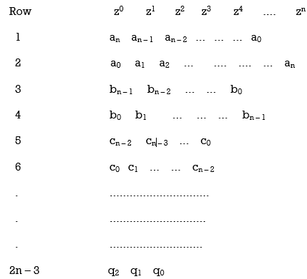
bk = 
k = 0, 1, 2, 3, ...., n – 1
ck = 
k = 0, 1, 2, 3, ...., n – 2
qk = 
This system will be stable if
1. |an| < a0
2. P(z)|z=1 > 0
3. P(z)|z=−1 > 0 for n even and P(z)|z=−1 < 0 for n odd
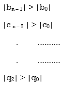
4.
Q2) The characteristic equation: P(z) = z4− 1.2z3 + 0.07z2 + 0.3z − 0.08 = 0 Thus, a0 = 1, a1 = −1.2, a2 = 0.07, a3 = 0.3, a4 = −0.08. By Jury test comment on stability.
A2) We will now check the stability conditions.
1. |an| = |a4| = 0.08 < a0 = 1 ⇒ First condition is satisfied.
2. P(1) = 1 − 1.2 + 0.07 + 0.3 − 0.08 = 0.09 > 0
Second condition is satisfied.
3. P(−1) = 1 + 1.2 + 0.07 − 0.3 − 0.08 = 1.89 > 0
Third condition is satisfied
Jury Table
b3 = 
= 0.0064 − 1 = −0.9936
b2 = 
= −0.08 × 0.3 + 1.2 = 1.176
Rest of the elements are also calculated in a similar fashion.
The elements are b1 = −0.0756
b0 = −0.204
c2 = 0.946
c1 = −1.184
c0 = 0.315.
One can see |b3| = 0.9936 > |b0| = 0.204 |c2| = 0.946 > |c0| = 0.315
All criteria are satisfied. Thus, the system is stable.
Q3) The characteristic equation: P(z) = z3− 1.3z2− 0.08z + 0.24 = 0 Thus a0 = 1, a1 = −1.3, a2 = −0.08, a3 = 0.24. Comment on stability.
A3) Stability conditions are:
- |a3| = 0.24 < a0 = 1 so First condition is satisfied.
- P(1) = 1 − 1.3 − 0.08 + 0.24 = −0.14 < 0 . The Second condition is not satisfied.
Since one of the criteria is violated, we may stop the test here and conclude that the system is unstable. P(1) = 0 or P(−1) = 0 indicates the presence of a root on the unit circle and in that case the system can at the most become marginally stable if rest of the conditions are satisfied.
Q4) Consider the system shown in Figure. Find out the range of K for which the system is stable.

A4)
G(z) = 
The closed loop transfer function

Characteristic equation: P(z) = z2 + (0.368K −1.368)z + 0.368 + 0.264K = 0
Since it is a second order system only 3 stability conditions will be there.
1. |a2| < a0
2. P(1) > 0 3. P(−1) > 0 since n = 2=even. This implies:
1. |0.368 + 0.264K| < 1
2.39 > K >−5.18
2. P(1) = 1 + (0.368K − 1.368) + 0.368 + 0.264K = 0.632K > 0 ⇒ K > 0
3. P(−1) = 1 − (0.368K − 1.368) + 0.368 + 0.264K = 2.736 − 0.104K > 0 ⇒ 26.38 > K
Combining all, the range of K is found to be 0 < K < 2.39.
If K = 2.39, system becomes critically stable.
The characteristics equation becomes
z2− 0.49z + 1 = 0
z = 0.244 ± j0.97
Sampling period T = 1 sec.
wd = (ws/2π) ∠z = (2π/2π) tan−1 (0.97/0.244) = 1.324 rad/sec
The above frequency is the frequency of sustained oscillation.
Bilinear Transformation:
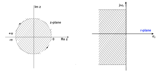
In z-domain for the system to be stable the roots of the characteristic equation must lie within the unit circle. But the transform z=esT cannot be used because the periodicity of esT and multiple strips of left half of s-plane into which the interior of the unit circle maps.
The Bilinear transformation maps the interior of the unit circle in the z-plane into the left half of r-plane.
r=
z=
On the unit circle in the z-plane
z= - 180
- 180 to +180
r= =
= =tanhj
 =jtan
=jtan =j
=j r
r
 r=tan
r=tan
The characteristic equation is
an + an-1
 +………..+a1
 +a0=0
+a0=0
Q) Using bilinear transformation determine the characteristic equation of given open loop function in z-plane. G(s)=
Sol: G(s)=
=5[  ]
]
=5[  ]
]
=
The characteristic equation is given as
1+G(S)= +
+ =0
=0
z3-0.5z2+2.49z-0.496=0
Putting in equation below
The characteristic equation is
an + an-1
 +………..+a1
 +a0=0
+a0=0
 -0.5
-0.5 +2.49
+2.49 -0.496=0
3.5r3-2.5r2+0.5r+2.5=0
The system stability can be checked using Routh array
The characteristic equation in s-domain will be
1+G(s)=0
1+ =0
=0
s3+3s2+2s+5=0

First column no sign change. Hence, system is stable.
Singular Cases
When some or all of the elements of a row in the Jury table are zero, the tabulation ends prematurely. This situation is referred to as a singular case. It can be avoided by expanding or contracting unit circle infinitesimally by an amount  which is equivalent to move the roots of P(z) off the unit circle.
The transformation is
z1 = (1 +  )z
)z
Where  is a very small number. When
  is positive the unit circle is expanded and when
  is negative the unit circle is contracted. The difference between the number of zeros found inside or outside the unit circle when the unit circle is expanded or contracted is the number of zeros on the unit circle. Since (1 +
  )nzn∼= (1 + n
 )zn for both positive and negative
  , the transformation requires the coefficient of the zn term be multiplied by (1 + n
 ).
).
Q5) The characteristic equation: P(z) = z3 + 0.25z2 + z + 0.25 = 0 Thus, a0 = 1, a1 = 0.25, a2 = 1, a3 = 0.25. Comment on stability?
A5) We will now check the stability conditions.
1. |an| = |a3| = 0.25 < a0 = 1
First condition is satisfied.
2. P(1) = 1 + 0.25 + 1 + 0.25 = 2.5 > 0
Second condition is satisfied.
3. P(−1) = −1 + 0.25 − 1 + 0.25 = −1.5 < 0
Third condition is satisfied.
Jury Table
b2 = 
b1 = 
Thus, the tabulation ends here and we know that some of the roots lie on the unit circle. If we replace z by (1 +  )z,
)z,
The characteristic equation would become
(1 + 3 )z 3 + 0.25(1 + 2
 )z 2 + (1 +
  )z + 0.25 = 0
First three stability conditions are satisfied.

|b2| = |0.0625 − (1 + 6 + 9
+ 9 2 )| and |b0| = |1 + 3.875
 + 3
+ 3 2− 0.0625|. Since, when
  → 0 +,
1 + 6 + 9
+ 9 2> 1 + 3.875
 + 3
+ 3 2, thus |b2| > |b0| which implies that the roots which are not on the unit circle are actually inside it and the system is marginally stable.
Lead Lag
To overcome the disadvantages of lead and lag compensation, they are used together. As lead compensation does not provide phase margin but has fast response and lag compensation stabilize the system but does not provide enough bandwidth.
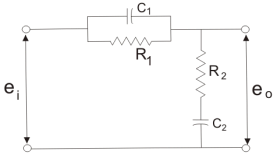
Fig 5. Lag-Lead Compensation
eo/ei = (1 + α ST1)/(1 + S T2)
T2)
Where, αT1 = R1C1
 T2=R2C2
We can say in the lag-lead compensation pole is more dominating than the zero and because of this lag-lead network may introduces positive phase angle to the system when connected in series.
For getting the required performance we need to adjust the design parameters and this is called compensation. To achieve the required output parameters a device called compensator is used. The compensators are mainly used to increase the steady state accuracy of system. These compensators minimise the overshoot. As these compensators are introduced in the system the transfer function changes and hence the performance specifications also change.
Phase Lag Compensation:
The phase of the output voltage lags the phase of the input voltage for applied sinusoidal input. The circuit diagram is shown below,
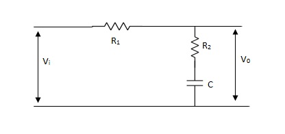
Fig 6. Phase Lag Compensation
Vo/Vi = 1 + ST/1 + SβT
Where, β = R1 + R2/R2, β> 1
T = R2C
w = 1/T upper corner frequency due to zero
w= 1/βT lower corner frequency due to pole
The mid frequency wm,
wm = 1/T√β
The maximum phase lead angle Φm
Φm = tan-11- β/2 √β
= sin-11 – β/1 + β
Phase – Lead Compensation:
The phase of output voltage leads the phase of input voltage for the applied sinusoidal input. The circuit diagram is shown below. The transfer function is given as,
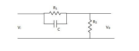
Fig 7. Phase Lead Compensation
Vo/Vi = α(1 + ST)/(1 + S α T)
Where, α = R2/R1 + R2 and α< 1
T = R1C
w = 1/T lower corner frequency due to zero.
w = 1/ αT upper corner frequency due to pole.
Mid frequency is given as,
wm = 1/T√ α
The maximum phase lead angle is φm
Φm = tan-1(1- α)/2√α = Sin-11- α/1 + α
For an nth order system with distinct eigenvalues the transfer function be
T(s)= =[b0sm+b1sm-1+….+bm-1s+bm/[sn+a1sn-1+……..+an-1s+an]
=K(s- 1)(s-
1)(s- 2)…….(s-
 m)/(s-
 1)(s-
1)(s- 2)……(s-
 n)
n)
= 
ck are residue poles at s=
If the transfer function has identical pair of poles and zeros at i=
i=  i
i
The effect of this cancellation of pole and zero on observability and controllability depends on the property of state variable.
- If the state variable is of the form below , then ci=0 will appear in control vector B and the state is uncontrollable.
 =
=  +
+  u
u
y=[1 1 1……..1] +b0u
+b0u
- On the other-hand if the state variables are of the form
 =
= +
+
y=[c1 c2 c3……..cn] +b0u
+b0u
Then then ci=0 will appear in output vector C and the state is shielded from observations.
- In LTI system if it has pole zero cancellation, the system will either be not controllable nor observable. But if the transfer function does not have any pole zero cancellations than the system can be represented by completely controllable and observable state model.
References:
1. Automatic Control Systems, Benjamin. C. Kuo, Prentice Hall of India, 7th Edition,1995.
2. Digital Control and State Variable Methods, M. Gopal, 2nd Edition, TMH, 2007.
3. Feedback and Control Systems, Stubberud, Schaum’s Outline Series, Tata McGraw-Hill, 2007.
4. Linear Control System Analysis and Design, John J. D’azzo & Constantine H.Houpis, Tata McGrow-Hill, Inc., 1995.
5. Modern Control Systems, Richard C. Dorf & Robert H. Bishop, Addison –Wesley, 1999.