Unit – 3
Statistics and Probability
A mean is a value which is representative of a set of data. Average value may also be termed as measures of central tendency. There are five types of averages in common.
(i) Arithmetic average or mean
(ii) Median
(iii) Mode
(iv) Geometric Mean
(v) Harmonic Mean
ARITHMETIC MEAN:
(a) If  are n numbers, then their arithmetic mean (A.M.) is defined by

This is known as direct method.
(b) Short cut method
Let a be the assumed mean, d the deviation of the variate x from a. Then

Example1. Find the arithmetic mean for the following distribution:
Class | 0-10 | 10-20 | 20-30 | 30-40 | 40-50 |
Frequency | 7 | 8 | 20 | 10 | 5 |
Solution: Let assumed mean (a) = 25
Class | Mid‐value
| Frequency |
|
|
40— 50 |
|
|
|
|
Total |
|
|
|
|

(c) Step deviation method
Let  be the assumed mean,
  the width ofthe class interval and

Example 2. Find the arithmetic mean of the data given in example 3 by step deviation method
Solution: Let 
Class | Mid‐value
| frequency
|
|
|
|
|
|
|
|
Total |
|
|
|
|

MEDIAN:
Median is defined as the measure of the central item when they are arranged in ascending or descending order of magnitude.
When the total number of the items is odd and equal to say  , then the value of
  th item gives the median.
When the total number of the frequencies is even, say  , then there are two middle items, and so the mean ofthe values of
  nth and
  th items is the median.
Example 3. Find the median of 6, 8, 9, 10, 11, 12, and 13.
Solution: Total number of items 
The middle item 
Median  Value of the 4th item
For grouped data, Median 
where  is the lower limit of the median class,
  is the frequency of the class,
  is the width ofthe class‐interval,
  is the total ofall the preceding frequencies of the median‐class and
  is total frequency ofthe data.
Example 4. Find the value of Median from the following data:
No. of days for which absent (less than) |
|
|
|
|
|
|
|
|
|
No. of students |
|
|
|
|
|
|
|
|
|
Solution: The given cumulative frequency distribution will first be converted into ordinary frequency as under
Class Interval | Cumulative frequency | Ordinary frequency |
0-5 5-10
15-20 20-25 25-35 30-35 35-40 40-45 | 29
465 582 634 644 650 653 655 | 29=29 224-29=195 465-224= 582-465=117 634-582=52 644-634=10 650-644=6 653-650=3 655-653=2 |
Median  size of
 or 327.
 Item
Item
327.  Item lies in 10‐15 which is the median class.

Where stands for lower limit ofmedian class,
 Stands for the total frequency,
 Stands for the cumulative frequency just preceeding the median class,
  stands for class interval
 Stands for frequency for the median class.
Median 

MODE
Mode is defined to be the size of the variable which occurs most frequently.
Example 5: Find the mode of the following items:
 .
.
Solution: 6 occurs 5 times and no other item occurs 5 or more than 5 times, hence the mode is 6.
For grouped data, 
where  is the lower limit of the modal class,
  is the frequency of the modal class,
  is the width of the class,
  is the frequency before the modal class and
  is the frequency after the modal class.
Empirical formula
Mean‐ Mode  [Mean
[Mean 
Example 6. Find the mode from the following data:
Age | 0-6 | 6-12 | 12-18 | 18-24 | 24-30 | 30-36 | 36-42 |
Frequency | 6 | 11 | 25 | 35 | 18 | 12 | 6 |
Solution:
Age | Frequency | Cumulative frequency |
0-6 6-12 12-18
24-30 30-36 36-42 | 6 11 25 35
12 6 | 6 17 42 77 95 107 113 |
Mode


GEOMETRIC MEAN
 , ,
, , be
be  values of variates
  , then the geometric mean

Example 7. Find the geometric mean of 4, 8, 16.
Solution:  .
.
HARMONIC MEAN
Harmonic mean of a series of values is defined as the reciprocal of the arithmetic mean of their reciprocals. Thus  be the harmonic mean, then

Example 8: Calculate the harmonic mean of 4, 8, 16.
Solution:


It is defined as the positive square root of the arithmetic mean of the square of the deviation of the given values from their arithmetic mean. It is denoted by symbol  .
.

Where  is A.M of the distribution
 . We have more formulae to calculate standard deviation.


1. Calculate S.D for the following distribution.
Wages in rupees earned per day | 0-10 | 10-20 | 20-30 | 30-40 | 40-50 | 50-60 |
No. of Labourers | 5 | 9 | 15 | 12 | 10 | 3 |
Solution:
Wages earned C.I | Mid value | Frequency |
|
|
|
52 | 5 | 5 | -2 | -10 | 20 |
153 | 15 | 9 | -1 | -9 | 9 |
25 | 25 | 15 | 0 | 0 | 0 |
35 | 35 | 12 | 1 | 12 | 12 |
45 | 45 | 10 | 2 | 20 | 40 |
55 | 55 | 3 | 3 | 9 | 27 |
Total | - |
|
|
|
|
Using formula,


2. Fluctuations in the aggregate of marks obtained by two groups of students are given below.
Group A | 518 | 519 | 530 | 530 | 530 | 544 | 518 | 550 | 527 | 527 | 531 | 550 | 550 | 529 | 528 |
Group B | 825 | 830 | 830 | 819 | 814 | 814 | 844 | 842 | 826 | 826 | 832 | 835 | 835 | 840 | 840 |
Solution:
First we represent the data in frequency distribution from group A
|
|
|
|
|
|
518 519 527 528 529 530 531 542 544 550 | 2 1 2 1 1 2 1 1 1 3 | -12 -11 -3 -2 -1 0 1 12 14 20 | 144 121 9 4 1 0 1 144 196 400 | -24 -11 -6 -2 -1 0 1 12 14 60 | 288 121 18 4 1 0 1 144 196 1200 |
Total |
|
|
|
|
|


For group B,
|
|
|
|
|
|
814 819 825 826 830 832 835 840 842 844 | 2 1 1 1 2 1 2 2 2 1 | -16 -11 -5 -4 0 2 5 10 12 14 | 256 121 25 16 0 4 25 100 144 196 | -24 -11 -6 -2 -1 0 1 12 14 60 | 288 121 18 4 1 0 1 144 196 1200 |
Total |
|
|
|
|
|


 Coefficient of variation
Formula for calculate Arithmetic Mean (A.M)


3. Calculate coefficient variation for the following frequency distribution.
Wages in Rupees earned per day | 0-10 | 10-20 | 20-30 | 30-40 | 40-50 | 50-60 |
No. of Labourers | 5 | 9 | 15 | 12 | 10 | 3 |
Solution:
We already calculated
 ….. (refer last Ex.)
Now, A.M 

A.M 
 Coefficient of Variation


4. Refer Question – 2 Calculate the coefficient of variation
Solution:
As we calculate,
σ for Group A σA=11.105
Now A.M 

A.M 
Coefficient of Variation


Same for Group B,

Now, 


Coefficient of Variation


The rth moment of a variable x about the mean x is usually denoted by is given by

The rth moment of a variable x aboutany point a is defined by


Relation between moments about mean and moment about any point:

 where
where and
and 


In particular


Note. 1. The sum of the coefficients of the various terms on the right‐hand side is zero.
2. The dimension of each term on right‐hand side is the same as that of terms on the left.
MOMENT GENERATING FUNCTION
The moment generating function of the variate  about
about  is defined as the expected value of
  and is denoted
  .
.


where  , ‘ is the moment of order
  about
about 
Hence  coefficient of
  or
or 
again  )
) 
Thus the moment generating function about the point  moment generating function about the origin.
Skewness denotes the opposite of symmetry. It is lack of symmetry. In a symmetrical series, the mode, the median, and the arithmetic average are identical.
Coefficient of skewness 
KURTOSIS: It measures the degree of peakedness of a distribution and is given by Measure of kurtosis.


Negative skewness Positive skewness
A.Mesokurtic
B.Leptokurtic
C. Playkurtic

If  , the curve is normal or mesokurtic.
If  , the curve is peaked or leptokurtic.
If  , the curve is flat topped or platykurtic
Whenever two variables x and y are so related that an increase in the one is accompanied by an increase or decrease in the other, then the variables are said to be correlated.
For example, the yield of crop varies with the amount of rainfall.
If an increase in one variable corresponds to an increase in the other, the correlation is said to be positive. If increase in one corresponds to the decrease in the other the correlation is said to be negative. If there is no relationship between the two variables, they are said to be independent.
Perfect Correlation: If two variables vary in such a way that their ratio is always constant, then the correlation is said to be perfect.
KARL PEARSON’S COEFFICIENT OF CORRELATION:
 between two variables x and y is defined by the relation

Where, X = x – , Y = y –
i.e. X, Y are the deviations measured from their respective means,

Example: Ten students got the following percentage of marks in Economics and Statistics
Calculate the co-efficient of correlation.
Roll No. |
|
|
|
|
|
|
|
|
|
|
Marks in Economics |
|
|
|
|
|
|
|
|
|
|
Marks in Statistics |
|
|
|
|
|
|
|
|
|
|
Solution: Let the marks oftwo subjects be denoted by  and
and  respectively.
Then the mean for  marks
marks  and the mean ofy marks
If  and
and are deviations of x’s and
 ’s from their respective means, then the data may be arranged in the following form:
|
|
|
|
|
|
|
78 | 84 | 13 | 18 | 169 | 324 | 234 |
36 | 51 | -29 | -15 | 841 | 225 | 435 |
98 | 91 | 33 | 25 | 1089 | 625 | 825 |
25 | 60 | -40 | -6 | 1600 | 36 | 240 |
75 | 68 | 10 | 2 | 100 | 4 | 20 |
82 | 62 | 17 | -4 | 289 | 16 | -68 |
90 | 86 | 25 | 20 | 625 | 400 | 500 |
62 | 58 | -3 | -8 | 9 | 64 | 24 |
65 | 53 | 0 | -13 | 0 | 169 | 0 |
39 | 47 | -26 | -19 | 676 | 361 | 494 |
650 | 660 | 0 | 0 | 5398 | 2224 | 2704 |
Here  ,
,  ,
, 


Solution: Let  be the ranks of
  individuals corresponding to two characteristics.
Assuming nor two individuals are equal in either classification, each individual takes the values 1, 2, 3,  and hence their arithmetic means are, each

Let  ,
,  ,
,  ,
,  be the values of variable
  and
and  ,
,  ,
,  those of
Then 
where and y are deviations from the mean.


Clearly,  and
and 


SPEARMAN’S RANK CORRELATION COEFFICIENT:

where denotes rank coefficient of correlation and
  refers to the difference ofranks between paired items in two series.
Example: Compute Spearman’s rank correlation coefficient r for the following data:
Person | A | B | C | D | E | F | G | H | I | J |
Rank Statistics | 9 | 10 | 6 | 5 | 7 | 2 | 4 | 8 | 1 | 3 |
Rank in income | 1 | 2 | 3 | 4 | 5 | 6 | 7 | 8 | 9 | 10 |
Solution:
Person | Rank Statistics | Rank in income |
|
|
A | 9 | 1 | 8 | 64 |
B | 10 | 2 | 8 | 64 |
C | 6 | 3 | 3 | 9 |
D | 5 | 4 | 1 | 1 |
E | 7 | 5 | 2 | 4 |
F | 2 | 6 | -4 | 16 |
G | 4 | 7 | -3 | 9 |
H | 8 | 8 | 0 | 0 |
I | 1 | 9 | -8 | 64 |
J | 3 | 10 | -7 | 49 |


Example: If X and Yare uncorrelated random variables,  the
the  of correlation between
  and
and 
Solution:
Let  and
and 
Then 
Now 
Similarly 
Now 


Also 


 (As
(As  and
and  are not correlated, we have
  )
)
Similarly 


REGRESSION
If the scatter diagram indicates some relationship between two variables  and
and , then the dots of the scatter diagram will be concentrated round a curve. This curve is called the curve ofregression. Regression analysis is the method used for estimating the unknown values of one variable corresponding to the known value of another variable.
LINE OF REGRSSION
When the curve is a straight line, it is called a line of regression. A line of regression is the straight line which gives the best fit in the least square sense to the given frequency.
Example: Find the correlation  betweenx and
  , when the lines ofregression are:
  and
and 
Solution: Let the line of regression ofx on  be
be 
Then, the line ofregression ofy on  is
is 

and
 which is not possible. So our choice of regression line is incorrect.
The regression line ofx on  is
is 
And, the regression line ofy on  is
is 

And 

Hence the correlation coefficient between  and
and  is
is 
Example: The following regression equations were obtainedfrom a correlation table:

Find the value of
(a) The correlation coefficient,
(b) The mean  and
and
(c) The mean of
Solution: 

(a) From (1), 
(b) From (2), 
From (3) and (4)


Coefficient of correlation 

(b) (1) and (2) pass through the point  .
.
 (5)
(5)
 (6)
(6)
On solving (5) and (6), we get

In addition to study the reliability of regression estimates we require to know the standard error.


2. The Standard error of Regression estimate of  on
on  is
is

1. Discuss the Reliability of Regression Estimates:
A | 45 | 38 | 59 | 64 | 72 |
B | 60 | 48 | 82 | 93 | 45 |
Solution:
For A,
| 45 | 38 | 59 | 64 | 72 |
|
| 2025 | 1444 | 3481 | 4096 | 5184 |
|


For B,
| 60 | 48 | 82 | 93 | 45 |
|
| 2025 | 1444 | 3481 | 4096 | 5184 |
|


Now,
| 45 | 38 | 59 | 64 | 72 |
|
| 60 | 48 | 82 | 93 | 45 |
|
| 2700 | 1824 | 4838 | 5952 | 3240 |
|


The standard error of Regression of estimates of y on x is


 …. (Standard error of Regression of estimates of y on x is)

3.8 Probability
Let Aand Bbe two events of a sample space Sand let  . Then conditional probability of the event A, given B, denoted by
 is defined by –

Theorem: If the events Aand Bdefined on a sample space S of a random experiment are independent, then

Example1: A factory has two machines A and B making 60% and 40% respectively of the total production. Machine A produces 3% defective items, and B produces 5% defective items. Find the probability that a given defective part came from A.
Solution: We consider the following events:
A: Selected item comes from A.
B: Selected item comes from B.
D: Selected item is defective.
We are looking for . We know:

Now,

So we need


Since, D is the union of the mutually exclusive events  and
and  (the entire sample space is the union of the mutually exclusive events A and B)


Example2: Two fair dice are rolled, 1 red and 1 blue. The Sample Space is
S = {(1, 1),(1, 2), . . . ,(1, 6), . . . ,(6, 6)}.Total -36 outcomes, all equally likely (here (2, 3) denotes the outcome where the red die show 2 and the blue one shows 3).
(a) Consider the following events:
A: Red die shows 6.
B: Blue die shows 6.
Find ,
,  and
and  .
.
Solution:


NOTE:  so
so  for this example. This is not surprising - we expect A to occur in
  of cases. In
  of these cases i.e. in
  of all cases, we expect B to also occur.
(b) Consider the following events:
C: Total Score is 10.
D: Red die shows an even number.
Find  ,
,  and
and  .
.
Solution:


NOTE:  so,
so, .
.
Why does multiplication not apply here as in part (a)?
Answer: Suppose C occurs: so the outcome is either (4, 6), (5, 5) or (6, 4). In two of these cases, namely (4, 6) and (6, 4), the event D also occurs. Thus
Although , the probability that D occurs given that C occurs is
  .
.
We write , and call
  the conditional probability of D given C.
NOTE: In the above example

Example3: Three urns contain 6 red, 4 black; 4 red, 6 black; 5 red, 5 black balls respectively. One of the urns is selected at random and a ball is drawn from it. If the ball drawn is red find the probability that it is drawn from the first urn.
Solution:
 :The ball is drawn from urnI.
 : The ball is drawn from urnII.
 : The ball is drawn from urnIII.
R:The ball is red.
We have to find 

Since the three urns are equally likely to be selected

Also,


From (i), we have

If  be any continuous random variable then the p.d.f
  then a function
  is said to be the P.D.F if

Here,  Random Variable
 Event
Event
 P.D.F
P.D.F
 P.M.F (discrete variable)
 Constant density function
Properties


1. If 
Find (i)  (ii)
(ii)  (iii)
(iii) 
Solution:
(i) Condition of P.D.F


(ii)


(iii) 


The Normal Distribution:
The normal distribution is sometimes informally called the bell curve.
The probability density of the normal distribution is:

 is mean or expectation of the distribution
 is the variance
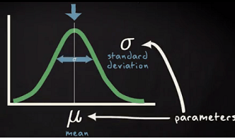
Properties of a normal distribution:
Binomial Distribution:
A distribution is said to be binomial distribution if the following conditions are met.
If all the above conditions met then the binomial distribution describes the probability of X successes in n trials.
A classic example of the binomial distribution is the number of heads (X) in n coin tosses.
The Notation for a binomial distribution is
X ~ B (n, π)
which is read as ‘X is distributed binomial with n trials and probability of success in one trial equal to π ’.
Formula for Binomial Distribution:
Using this formula, the probability distribution of a binomial random variable X can be calculated if n and π are known.

n! is called ‘n factorial’ = n(n-1)(n-2) . . .(1)
P(X) = #of Scenario * Single Scenario
The first factorial terms gives the number of scenario and the second term describes the probability of success to power of number of successes and probability of failure to the power of number of failures.
Another probability distribution for discrete variables is the Poisson distribution. The Poisson distribution is used to determine the probability of the number of events occurring over a specified time or space. This was named for Simeon D. Poisson, 1781 – 1840, French mathematician.
Examples of events over space or time: -number of cells in a specified volume of fluid
-number of calls/hour to a help line
-number of emergency room beds filled/ 24 hours
Like the binomial distribution and the normal distribution, there are many Poisson distributions.
The probability that there are exactly X occurrences in the specified space or time is equal to

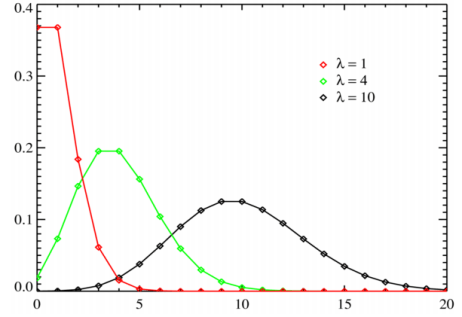
The horizontal axis is the index X. The function is defined only at integer values of X. The connecting lines are only guides for the eye and do not indicate continuity. Notice that as λ increases the distribution begins to resemble a normal distribution.
Normal Distribution Probability Calculation:
Probability density function or p.d.f. specified the probability per unit of the random variable. Here is an example of a p.d.f. of the daily waiting time by the taxi driver of Uber Taxi Company. In the X axis, daily waiting time and Y-axis probability per hour has been shown.
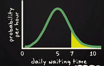
If one Uber taxi driver want to know the probability to wait more than 7 hours in a day? Then he will be interested in the yellow surface arear shown above. On basis of this graph you can estimate the area. Same thing you can get form below
Cumulative probability curve.
.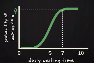
Probability to wait more than 7 hours will be calculated using complementary rule 1- P. Because corresponding to 7 in X axis we marked the probability is P and we are interested in more than 7 hours. So, P should be subtracted from 1 to get desired result.
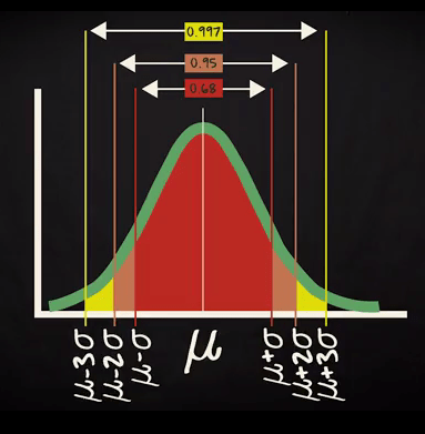
Bell Shaped Distribution and Empirical Rule:If distribution is bell shape then it is assumed that about 68% of the elements have a z-score between -1 and 1; about 95% have a z-score between -2 and 2; and about 99% have a z-score between -3 and 3.
Assume the time you spend in week days by traveling has given by a normal distribution with mean= 40 mins and SD= 10 mins.
What will be your range of travel time for 95 % of your week days?
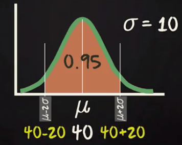
As you know 95 % will come within 2 standard deviation of your mean. So, the range will be (40-20) = 20 to (40+20) =60 mins.
Now another question you want to answer that what will be the probability to be travelling more than 50 mins?
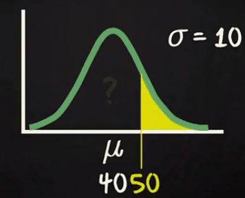
Actually you are interested in the yellow surface given in above diagram. You know that a normal distribution is symmetric. So, half of the probability located one side of the mean and another half located another side of the mean.
As SD =10. So, one standard deviation will be 30 to 50 range.
You already know for left side up 40 the probability is 0.5. Now if you calculate the probability from 40 to 50 range it will be half of 1 Standard deviation i.e. 0.68/2 = 0.34
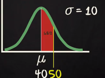
So the probability to travel less than 50 mins = 0.5 +. 0.34 = 0.84
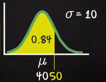
But you are interested in more than 50 mins traveling time so it will be 1- 0.84 =0.16
Chi – Square Test
 Observed Frequency
 Expected (Theoretical) Frequency
Then Chi – Square distribution is defined as

Where,  Total Frequency
Chi-Square ( ) Test: Working Rule
Step I:
Consider the null hypothesis ( ) and Alternative Hypothesis (
 )
)
Step II:
Consider expected frequency  corresponding to each cell.
Step III:
Calculate  distribution by the formula
 and calculate the degree of freedom(
 .
.
Step IV:
See the value of  from the table and the value calculate in step (3).
Step V:
If Calculated value of  <Tabulated value of
Then Null hypothesis  is accepted otherwise
  accepted.
Calculation of Expected frequency 2×4 Table
|
|
| Total |
|
|
|
|
|
|
|
|
Total |
|
|
|
Expected frequencies of cell (1,1) is given by


Calculation of Degree of freedom ( ):
):
Binomial Distribution 
Poisson’s Distribution
Normal Distribution

1. In a sample survey of public opinion answer to the question
(i) Do you drink?
(ii) Are you in favour of local option on sale of liquor?
Are tabulate below:
| Yes | No | Total |
Yes | 56 | 31 | 87 |
No | 18 | 6 | 24 |
Total | 74 | 37 | 111 |
Can you infer or not the local option on the safe of liquor is depend on individual drink?
(Given that the value of  for dof at 5% level of significance is 3.841)
Solution:
Step 1:
Null Hypothesis  . The option on the safe of liquor is not depend with the individual drinking.
Step 2:
Calculation of expected frequency (Theoretical Frequency)


Step 3:
Calculation of  distribution. We know that
 (1)
(1)


Decision:
Clearly calculated value of 
Tabulated value of  (3.841)
Null hypothesis is accepted.
Safe of liquor is not depending with the individual drink.
T – Test:
(i) T – Test is a small sample test
(ii) It is also called student T – Test.

(iii) Also called as Welch t – Test.
Uses of T – Test:


Reference Books


