3.1 Dimensional Homogeneity | unit 3 dimensional analysis and model studies boundary layer theory

Unit 3

Dimensional Analysis and Model Studies & Boundary layer Theory

3.1 Dimensional Homogeneity

A physical equation is a relationship between two or more physical quantities.

Any correct equation expressing a physical relationship between quantities must be dimensionally homogeneous and numerically equivalent.

Dimensional homogeneity states that every term in an equation when reduced to fundamental dimensions must contain identical powers of each dimension.

A dimensionally homogeneous equation applies to all systems of units.

In a dimensionally homogeneous equation, only quantities having the same dimensions can be added, subtracted, or equated.

P = w h

Dimensions of LHS = ML-1T-2

Dimensions of RHS = ML-2T-2×L = ML-1T-2

Dimensions of LHS = Dimensions of RHS

Hence, equation P= w h is dimensionally homogeneous; so it can be used in any system of units.

Applications of Dimensional Homogeneity:

It facilitates to determine the dimensions of a physical quantity.

It helps to check whether an equation of a physical phenomenon is dimensionally homogeneous or not.

It facilitates the conversion of units from one system to another.

3.2 Dimensional analysis using Buckingham’s Π- Method/Theorem

When a large number of physical variables are involved Rayleigh’s method of dimensional analysis becomes increasingly laborious and cumbersome.

Buckingham’s method is an improvement over the Rayleigh’s method.

Buckingham’s designated the dimensionless group by the letter Π. It is therefore often called Buckingham Π-Method.

Buckingham’s Π-Method states as follows:

“If there are n variables in a dimensionally homogeneous equation and if these variables contain fundamental dimensions (such as M, L, T, etc.) then the variables are arranged into (n-m) dimensionless terms.

These dimensionless terms are called Π – terms.”

Mathematically, if any variable X1, depends on independent variables, X2, X3, X4,…… Xn; the functional equation may be written as

-------- 1

Equation 1 can also be written as

-------- 2

It is a dimensionally homogeneous equation and contains n variables.

If there are m fundamental dimensions, then according to Buckingham’s Π – theorem, it [eqn] can be written in terms of number of Π – terms in which the number of Π terms is equal to (n-m).

Hence equation 2 becomes as

--------3

Each dimensionless – term is formed by combining m variables out of the total n variables with one of the remaining (n-m) variables.

These m variables which appear repeated in each of – terms are consequently called repeating variables and are chosen from among the variables such that they together involve all the fundamental dimensions and they do not form a dimensionless parameter.

Let in the above case X2, X3 and X4 are the repeating variables if the fundamental dimensions m(M, L, T) = 3, then each term is written as:

-------- 4

Where a1, b1, c1, a2, b2, c2, etc. are the constants, which are determined by considering dimensional homogeneity. These values are substituted in equation 4 and the values of are obtained. These values of Π’s are substituted in equation 3.

The final general equation for the phenomenon may then be obtained by expressing anyone of the Π – terms as a function of the other as:

3.3 Geometric similarity, Kinematic similarity & Dynamic similarity

Geometric Similarity:

For geometric similarity to existing between the model and the prototype, the ratios of corresponding lengths in the model and the prototype must be the same and the included angles between the corresponding sides must be the same.

Models that are not geometrically similar are known as a geometrically distorted model.

Lm = length of model

Hm = height of the model

Dm = diameter of the model

Am = area of the model

Vm = volume of the model

And LP, BP, HP, DP, AP, and VP = corresponding values of the prototype.

Then, for geometric similarity, we must have the relation:

Where Lr is called the scale ratio or the scale factor:

Kinematic similarity:

The kinematic similarity is the similarity of motion.

If at the corresponding points in the model and the prototype, the velocity or acceleration ratio is the same & velocity or acceleration vectors point in the same direction, the two flows are said to be kinematically similar.

(V1)m = velocity of the fluid at point 1 in the model.

(V2)m = velocity of the fluid at point 2 in the model,

(a1)m = acceleration of fluid at point 1 in the model

(a2)m = acceleration of fluid at point 2 in the model

And (V1)P, (V2)P, (a1)P (a2)P = corresponding values at the corresponding points of fluid, velocity, and acceleration in the prototype.

Then, for kinematic similarity, we must have

Similarly,

The direction of the velocities in the model and prototype should be the same.

The geometric similarity is a pre-requisite for kinematic similarity.

Dynamic Similarity

The dynamic similarity is the similarity of forces. The flows in the model and prototype are dynamically similar if, at all the corresponding points, identical types of forces are parallel and bear the same ratio.

In dynamic similarity, the force polygons of the two flows can be superimposed by a change in the force scale.

(Fi)m = inertia force at a point in the model,

(Fv)m = viscous force at the point in the model,

(Fg)m = gravity force at the point in the model

And (Fi)P, (Fv)P, (Fg)P = corresponding values of forces at the corresponding points in the prototype.

Then, for dynamic similarity we have

The direction of the corresponding forces at the corresponding points in the model and prototype should also be the same.

3.4 Important dimensionless Numbers (Reynolds No., Froude No., Euler No., Mach no. and Weber No) and their significance

Reynold’s Number (Re)

It is defined as the ratio of the inertia force to the viscous force.

Reynold’s Number, Re =

For pipe flow (where the linear dimension is taken as diameter d),

Reynold’s number signifies the relative predominance of the inertia to the viscous forces occurring in the flow systems.

Fraud’s Number (Fr)

It is defined as the square root of the ratio of the inertia force and the gravity force.

Mathematically,

Froude number governs the similarity of the dynamics of the flow situations; where the gravitational force is more significant and all other forces are comparatively negligible.

Euler’s Number (Eu)

It is defined as the square root of the ratio of the inertia force to the pressure force.

The Euler number is important in the flow problems/situations in which a pressure gradient exists.

Weber’s Number (We)

It is defined as the square root of the ratio of the inertia force to the surface tension force.

Mathematically,

This number assumes importance in the following flow situation:

i) The flow of blood in veins and arteries

ii) Liquid atomisation, and

iii) Capillary movement of water in soils

Mach Formula (M)

It is defined as the square root of the ratio of the inertia force to the elastic force.

Mathematically,

The Mach number is important in compressible flow problems at high velocities, such as high-velocity flow in pipes or motion of high-speed projectiles and missiles.

3.5 Model Laws (Reynold’s law and Froude’s Law)

To ensure dynamic similarity between the model and prototype it is necessary that the ratio of the corresponding forces acting at the corresponding points in the model and prototype be made equal.

It implies that dimensionless numbers should be the same for the model as well as the prototype.

This condition is difficult to be satisfied with all the dimensionless numbers.

Hence models are designed based on the force which is dominating the flow situation. The laws on which the models are designed for dynamic similarity are called model or similarity laws; these are

Reynolds Model Law

Inflow situations where in addition to inertia, viscous force is the other predominant force, the similarity of flow in the model and its prototype can be established if Reynolds number is the same for both the systems.

This is known as Reynolds law and according to this law,

Where, ρm = density of the fluid in the model

Vm = velocity of the fluid in the model,

Lm = length of the linear dimension of the model, and

µm = viscosity of the fluid in the model

and ρP, VP, LP, and µP are the corresponding values of density, velocity, linear dimension, and viscosity of the fluid in the prototype.

[

Following are some of the phenomenon for which Reynolds model law can be a sufficient criterion for similarity of flow in the model and the prototype:

The motion of airplanes,

The flow of incompressible fluid in closed pipes,

The motion of submarines completely underwater, and

Flow around structures and other bodies immersed completely under moving fluids.

Froude Model Law

When the gravitational force can be considered to be the only predominant force that controls the motion in addition to the inertia force, the similarity of the flow in any two such systems can be established if the Froude’s number of both the systems is the same.

This is known as Froude’s Model Law.

Some of the phenomenon for which the Froude Model Law can be sufficient criterion for dynamic similarity to be established in the model and the prototype are:

Free surface flows such as flow over spillways, sluices, etc.

The flow of jet from an office or nozzle;

Where waves are likely to be formed on the surface;

Where fluids of different mass densities flow over one another

Let, Vm = velocity of the fluid in the model

Lm = length (or linear dimension) of the model

gm = acceleration due to gravity (at a place where the model is tested)

and VP, LP, and gP are the corresponding values of the velocity, length, and acceleration due to gravity for the prototype.

Then according to Froude Law,

(Fr)m = (Fr)P

Or ------ 1

As the value of g at the site of mode testing will be practically the same as at the site of the proposed prototype, therefore gm = gP and the equation 1 values as

Where Lr = scale ratio for length

3.6 Concept of boundary layer

When a real fluid flows past a stationary solid boundary, a layer of fluid that comes in contact with the boundary surface adheres to it & the condition of no-slip occurs.

Thus the layer of fluid which cannot slip away from the boundary surface undergoes retardation.

This retarded layer further causes retardation for the adjacent layers of fluid, thereby developing a small region in the intermediate vicinity of boundary surface in which the velocity of the fluid increases rapidly from zero at the boundary surface & approaches the velocity of the mainstream.

The layer adjacent to the boundary is known as the boundary layer.

The boundary layer is formed whenever there is relative motion between the boundary & the fluid.

3.7 Development of the boundary layer on flat plate and factors affecting the growth

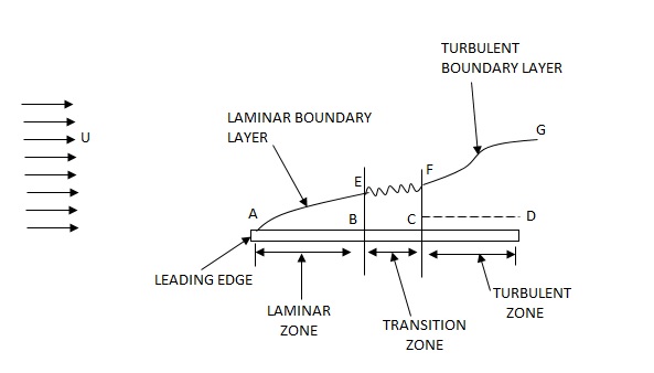
Laminar and turbulent boundary layer

Laminar Boundary Layer

Consider the flow of fluid having free stream velocity(U) over a smooth thin plate which is flat and placed parallel to the direction for a free stream of fluid as shown in the figure.

Let us consider the flow with zero pressure gradient on one side of the plate which is stationary.

The velocity of the fluid on the surface of the plate should be equal to the velocity of the plate. But the plate is stationary and hence the velocity of a fluid on the surface of the plate is zero. But at a distance away from the plate, the fluid is having a certain velocity.

Thus, a velocity gradient is set up in the fluid near the surface of the plate. This velocity gradient develops shear resistance, which retards the fluid.

Thus, the fluid with a uniform free stream velocity(u) is retarded in the vicinity of the solid surface of the plate and the boundary layer region begins at the sharp leading edge.

At subsequent points downstream the leading edge, the boundary layer region increases because the retarded fluid is further retarded.

This is also referred to as the growth of the boundary layer.

Near the leading edge of the surface of the plate, where the thickness is small, the flow in the boundary layer is laminar though the main flow is turbulent.

This layer of the fluid is said to be a laminar boundary layer. This is shown by AE in the figure.

Turbulent Boundary Layer

The thickness of the boundary layer will go on increasing in the downstream direction.

Then the laminar boundary layer becomes unstable and the motion of fluid within it is disturbed and irregular which leads to a transition from laminar to the turbulent boundary layer.

This short length over which the boundary layer flow changes from laminar to turbulent is called the transition zone. This is shown by distance BC in the figure.

Further downstream the transition zone, the boundary layer is turbulent and continues to grow in thickness. The layer of the boundary is called the turbulent boundary layer, which is shown by the portion FG in the figure.

3.8 Boundary Layer Thickness

Boundary-Layer Thickness ()

It is defined as the distance from the boundary of the solid body measured in the y-direction to the point, where the velocity of the fluid is approximately equal to 0.99 times the free stream velocity(u) of the fluid.

It is denoted by the symbol

1. = Thickness of laminar boundary layer,

2. = Thickness of turbulent boundary layer, and

3. = Thickness of laminar sublayer.

3.9 Displacement thickness, momentum, and energy thickness

Displacement Thickness()

It is defined as the distance, measured perpendicular to the boundary of the solid body, by which the boundary should be displaced to compensate for the reduction in flow rate on account of boundary layer formation.

It is denoted by

It is also defined as “The distance perpendicular to the boundary, by which the free stream is displaced due to the formation of boundary layer”.

Momentum Thickness (

Momentum thickness is defined as the distance, measured perpendicular to the boundary of the solid body, by which the boundary should be displaced to compensate for the reduction in the momentum of the flowing fluid on account of boundary layer formation.

It is denoted by

Energy Thickness ()

It is defined as the distance measured perpendicular to the boundary of the solid body, by which the boundary should be displaced to compensate for the reduction in kinetic energy of the flowing fluid on account of boundary layer formation.

It is denoted by

3.10 Laminar sub-layer

For turbulent flow analysis along a boundary, the flow is divided into two portions.

The first portion consists of a thin layer of fluid in the immediate neighbourhood of the boundary, where viscous shear stress predominates while the shear stress due to turbulence is negligible.

This portion is known as the laminar sub-layer.

It is denoted by

3.11 Local and mean drag coefficients

Local coefficient of drag (CD*)

It is defined as the ratio of the shear stress to the quantity

It is denoted by CD*

The average coefficient of Drag (CD)

It is defined as the ratio of total drag force to the quantity

It is also called the coefficient of drag and is denoted by CD.

where A= area of the surface (or plate)

V = free stream velocity

= mass density of fluid

3.12 Hydrodynamically smooth and Rough Boundaries

If K is the arrange height of the irregularities of the surface of a boundary, then in general the boundary is said to be rough if the value of K is high and smooth if K is low.

For proper classification of smooth and rough boundaries, besides the boundary characteristics, the fluid and fluid characteristics need to be considered.

As shown in fig: when the average height K of the irregularities is much less than the thickness of the laminar sublayers

the flow outside the laminar sublayer is turbulent; the eddies of various sizes present, try to penetrate the laminar sub-layer.

These eddies cannot reach the surface irregularities due to greater thickness of the laminar sublayer and so the boundary acts as a smooth boundary.

As the Reynolds numbers (Re) increases the thickness of the sublayer decreases the irregularities will then project through laminar sublayer and eventually the laminas sublayer is destroyed completely.

Subsequently, the eddies will come in contact with the surface irregularities and there will be a large amount of energy loss.

This type of boundary is known as hydrodynamically rough boundary.

Through experiment Nikuradse found that the boundary behaves as :

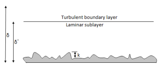
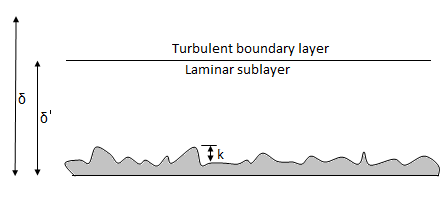
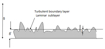
i) Hydrodynamically smooth boundary, when () < 0.25

ii) Hydrodynamically rough boundary, when () > 6.0

iii) Boundary in transition, when 0.25 < () < 6.0

3.13 Boundary Layer separation and methods to control separation

Separation of boundary layer

When a solid body is immersed in a flowing fluid, a thin layer of fluid called the boundary layer is formed adjacent to the solid body.

Along the length of the solid body the thickness of the boundary layer increases.

The fluid layer adjacent to the solid surface has to do work against surface frictional at the expense of its kinetic energy.

This loss of kinetic energy is recovered from the immediate fluid layer in contact with the layer adjacent to the solid surface through the momentum exchange process.

Thus, the velocity of the layer goes on decreasing along the length of the solid body.

At a certain point, a stage may come when the boundary layer may not be able to keep sticking to the solid body if it cannot provide kinetic energy to overcome the resistance offered by the solid body. The boundary layer will be separated from the surface.

This phenomenon is called boundary layer separation.

The point on the body at which the boundary layer is on the verge of separation from the surface is called the point of separation.

Methods of preventing the separation of the boundary layer

The following are the methods of preventing the separation of the boundary layer:

The motion of solid boundary:

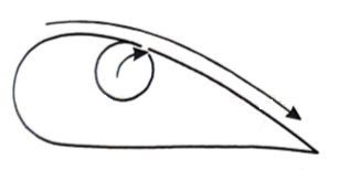
By rotating a circular cylinder lying in a stream of fluid so that the upper side of the cylinder where the fluid, as well as the cylinder, move in the same direction, the boundary layer does not form.

2. Acceleration of fluid in the boundary layer:

This method of controlling separation consists of supplying additional energy to particles of fluid which are being retarded in the boundary layer. This may be achieved either by injecting the fluid into the region of the boundary layer from the interior of the body with the help of some available device as shown in the figure or by diverting a portion of fluid of the mainstream from the region of high pressure to the retarded region of boundary layer through a slot provided in the body.

3. The suction of fluid from the boundary layer:

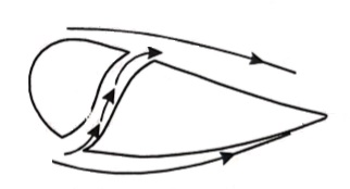
In this method, the slow-moving fluid in the boundary layer is removed by suction through slots or a porous surface as shown in the figure.

4. Streamlining of the body shapes:

By the use of suitably shaped bodies, the point of transition of the boundary layer from laminar to turbulent can be moved downstream which results in the reduction of the skin friction drag. Furthermore, by streamlining the body shapes the separation may be eliminated.

5. Supplying additional energy from a blower.

6. Rotating boundary in the direction of flow.

7. Providing small divergence in a diffuser.

8. Providing guide blades in a bend.

9. Providing a tripwire ring in the laminar region for the flow over a sphere.

Reference books:

1. Engineering Fluid Mechanics by R. J. Garde and A.J Mirajgaonkar, Pub: SCITECH Publications( India )Pvt.Ltd, Chennai

2. Fluid Mechanics and its Applications, Vijay Gupta, Santosh K Gupta, New Age International Pvt. Ltd, New Delhi,

3. Fluid Mechanics, Fundamentals, and applications by Yunus. A Cengel and John.M Cimbala, Mc Graw Hill International, New Delhi.

4. Fluid Mechanics by Streeter, Wylie, and Bedford – Pub: McGraw Hill International, New Delhi.

5. Open Channel Hydraulics by Ven Tee Chow, Pub: Mcgraw- Hill Book Company- Koga.

6. A Text-Book of Fluid Mechanics and Hydraulic Machines- by Dr. R K Rajput Pub: S Chand and Co Ltd. New Delhi

Sign Up

Index

Notes

Highlighted

Underlined

Browse by Topics

Notes

Highlighted

Underlined