UNIT-5

TREES

5.1 Introduction

Graph G is called a tree if G is connected and contains no cycles.

Graph whose connected components are trees: forest

A tree is a connected undirected graph with no simple circuits.

A (not-necessarily-connected) undirected graph without simple circuits is called a forest.

5.2 Properties of trees

A rooted tree is a tree in which one vertex has been designated as the root and every edge is directedaway from the root.

Suppose that T is a rooted tree. If v is a vertex in T other than the root, the parent of v is the uniquevertex u such that there is a directed edge from u to v.

If u is the parent of v, then v is called a child of u.

Vertices with the same parent are called siblings.

The ancestors of a vertex other than the root are the vertices in the path from the root to this vertex, excluding the vertex itself and including the root.

The descendants of a vertex v are those vertices that have v as an ancestor.

A vertex of a tree is called a leaf if it has no children.

Vertices that have children are called internal vertices.

If a is a vertex in a tree, the sub tree with a as its root is the sub graph of the tree consisting of a andits descendants and all edges incident to these descendants.

A rooted tree is called an m-ary tree if every internal vertex has no more than m children. The treeis called a full m-ary tree if every internal vertex has exactly m children.

5.3 Binary search tree

Binary Tree

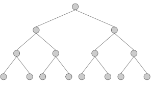
An m-ary tree with m = 2 is called a binary tree.

Ordered Root Tree

An ordered rooted tree is a rooted tree where the children of each internal vertex are ordered.

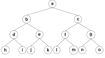
Left and Right Child

In an ordered binary tree, the first child is called the left child and the second child is called the

Rightchild.

Left and Right Sub tree

The tree rooted at the left child is called the left sub treeand the tree rooted at the right child is

Called the right sub tree.

Example 1: Every binary tree has an odd no. Of vertices.

Solution: let T = (V, E) be a binary tree.

A part from the root every vertex in a binary tree is an odd degree.

w.k.t., there must be an even no. of vertices such odd degree.

When the root which of odd degree is added to this even no. Of vertices i.e.,

Even no. of vertices and one root vertex, we have odd no. Of vertices.

Therefore, every binary tree has odd no. of vertices

Note: let a tree has ‘n’ vertices and ‘m’ pendent vertices, then the no. of internal vertices of degree 3 is n-(m+1)

 Example 2: prove that there are pendent vertices in any binary tree with ‘n’ vertices.

Solution: suppose T = (V, E) be a binary tree with ‘n’ vertices. Let ‘m’ be the two no. of pendent vertices in T. Then T has (n-(m+1)) no. of internal vertices of degree 3

So, the sum of degree of all vertices in T is 3(n-m-1) + m+2….(1)

Since T is tree with ’n’ vertices then it has (n-1) edges.

So, the degree sum of ‘n’ vertices in T is given by

(2)

From (1) and (2)

  The no.of pendent vertices in binary tree is 

5.4 Tree traversal

Traversal is a process to visit all the nodes of a tree and may print their values too. Because, all nodes are connected via edges (links) we always start from the root (head) node. That is, we cannot randomly access a node in a tree. There are three ways which we use to traverse a tree −

Generally, we traverse a tree to search or locate a given item or key in the tree or to print all the values it contains.

Example: find the tree traversal for the following binary tree.

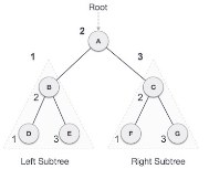
Solution: we follow the known three steps to get the final tree traverse i.e.,

Step-1: In-order Traversal

In this traversal method, the left sub tree is visited first, then the root and later the right sub-tree. We should always remember that every node may represent a sub tree itself.

If a binary tree is traversed in-order, the output will produce sorted key values in an ascending order.

We start from A, and following in-order traversal, we move to its left subtree B. B is also traversed in-order. The process goes on until all the nodes are visited.

The required tree-traversal is the following order.

D → B → E →A→ F → C → G

Algorithm

Step-1: Recursively traverse left sub tree

Step -2: visit root node

Step-3: Recursively traverse right sub-tree.

We will continue this process until all nodes are traversed.

Step-2:Pre-order Traversal

In this traversal method, the root node is visited first, then the left subtree and finally the right subtree.

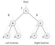
We start from A, and following pre-order traversal, we first visit A itself and then move to its left subtree B. B is also traversed pre-order. The process goes on until all the nodes are visited.

The required tree traversal is the following order.

A → B → D → E → C → F → G

Algorithm:

Step-1: Visit root node.

Step-2: Recursively traverse left sub-tree.

Step-3:Recursively traverse right sub-tree.

Step-3:Post-order Traversal

In this traversal method, the root node is visited last, hence the name. First we traverse the left subtree, then the right subtree and finally the root node.

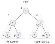
We start from A, and following Post-order traversal, we first visit the left sub-tree B. B is also traversed post-order. The process goes on until all the nodes are visited. The output of post-order traversal of this tree will be −

D → E → B → F → G → C → A

Algorithm:

Step-1: Recursively traverse left sub-tree.

Step-2: Recursively traverse right sub-tree.

Step-3: Visit root node.

5.5 Decision tree

At first, a decision tree appears as a tree-like structure with different nodes and branches. When you look a bit closer, you would realize that it has dissected a problem or a situation in detail. It is based on the classification principles that predict the outcome of a decision, leading to different branches of a tree. It starts from a root, which gradually has different decision nodes. The structure has terminating nodes in the end.

Ideally, a decision tree can be used in almost every sector. This is because we can take any real-world or hypothetical instance and represent it using a decision tree diagram. To further understand what a decision tree is, let’s consider this example. It asks a simple question – whether to buy a new software or not. If we buy a new tool, then it further leads to the comparison between the two options. If not, then we can either continue using the present software or borrow a friend’s tool.

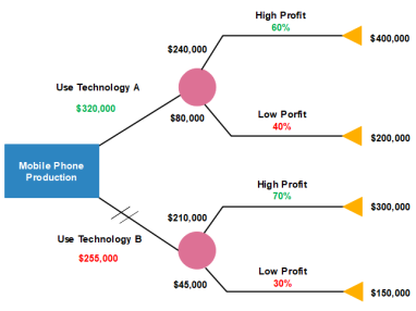
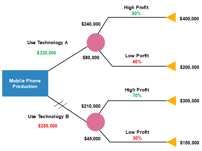
Example1: Draw the decision tree for the below data.

A company has mobile production process by using two-technologies A and B namely. Where the details are given below

Technology A: The cost for using this technology is $ 320,000 and we have two processes which gain 60 % and 40 % profit respectively.

By using decision tree classify the following.

Technology B:

Solution: The cost for using this technology is $255,000 and we have two processes which gain 70 % and 30 % profit respectively.

Solution:

Example 2: Draw a decision tree for the following data..

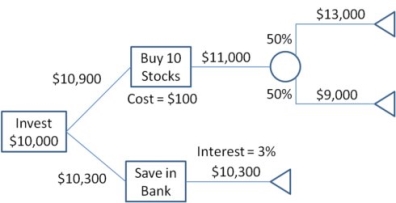
A person gets $ 10,300 by saving in bank and conversely he gets $ 13000 and @ 9,000 by buying stocks so draw the decision tree for the given data and express which method is best to earn more income

Solution:

5.6 Prefix codes and Huffman coding, cut sets.

Prefix codes:

Suppose

And given code is 0100 now the answer may be

ABAB OR ADB OR DAB

So we cannot say which can be considered in order to avoid such confusion pre-fix codes helps us to de-code such kind of problems.

In discrete mathematics

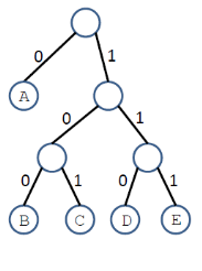
1. Each edge is labeled by a bit,

2. Each leaf a character

3. Labels on root-to-leaf path code word for the character.

Example:

E.g.,

Given the frequencies of each character, design the optimal pre-fix code whose en-coded text requires the least storage. We want to find a pre-fix code tree that corresponds to an optimal pre-fix code.

Solution:

Step 1: In an optimal pre-fix code tree, each internal node must have two children.

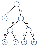
The above tree is not an optimal pre-fix code tree.

Step 2: To get an optimal pre-fix code tree the leaves must be corresponding to the least frequent characters which are siblings, and the leaves are farthest from the root.

For this we consider an optimal pre-fix code tree.

Let y and z be the least frequent characters.

Let x be a character whose leaf is farthest from the root( its sibling g must be a leaf for some character ‘x’).

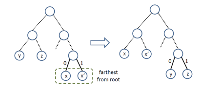
Is the required optimal pre-fix tree.

Huffman coding:

Based on pre-fix code observations, we get a way to obtain an optimal pre-fix code:

1.Find the least frequent characters X and Y.

2. Form two leaves for X and Y, and join them with a common parent p.

3. Replace   X and Y by a common character c

4. Recursively find the optimal pre-fix code tree for the new text (and replace the leaf for c with p, x, y).

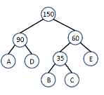
Example 2: suppose the relative frequencies as follows:

Step-1:                               Step-2:                                         Step-3:

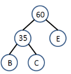
Step-4: finally the Huffman coding is represented in the below tree.

Cut sets:Let 'G'= (V, E) be a connected graph. A subset E' of E is called a cut set of G if deletion of all the edges of E' from G makes G disconnect.

If deleting a certain number of edges from a graph makes it disconnected, then those deleted edges are called the cut set of the graph.

Example:

Take a look at the following graph. Its cut set is E1 = {e1, e3, e5, e8}.

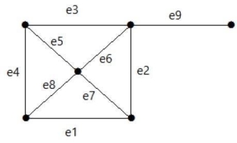
Solution:

After removing the cut set E1 from the graph, it would appear as follows −

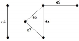
Similarly there are other cut sets that can disconnect the graph –

5.7 Spanning trees and Minimum spanning tree

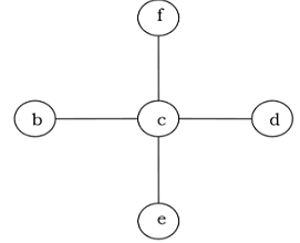
The tree which includes all the vertices of the connected undirected graph G very minimally is known as a spanning tree. A single graph can have many spanning trees.

Example:

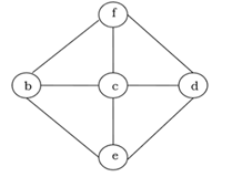
After spanning the above graph becomes

Minimum spanning trees:

We find minimum spanning trees by using Kruskal’s or Prim’s algorithms.

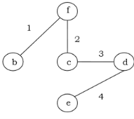
When the assigned weight is less than or equal to the weight of all possible spanning tree of weighted, connected and undirected graph G, such a spanning tree is called as Minimum Spanning Tree (MST). The weight of the spanning tree is calculated by the total of all the weights that are assigned to each edge of the spanning tree.

Example:

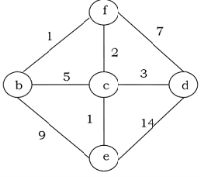
We get the minimum spanning tree as follow

5.8 Kruskal’s and Prim’s algorithms

KRUSKAL’S ALGORITHM:

An algorithm that is used for finding the minimum spanning tree of a connected weighted graph is known as Kruskal’s algorithm. A tree among the graph is identified which includes every vertex and where the total weight of all the edges in the tree is less than or equal to the spanning tree.

Algorithm

Step 1– All the edges of the given graph G (V,E) are arranged in the non-decreasing order in accordance with the weight of the edge.

Step 2 – The smallest weighted edge from the graph is chosen and is checked if it forms a spanning tree earlier.

Step 3 – This edge is included to the spanning tree if there is no cycle, or else it is discarded.

Step 4− Repeat Step 2 and Step 3 until (V−1) number of edges are left in the spanning tree.

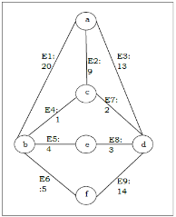
Example 1:For instance, identify the minimum spanning tree from the following graph G by using the Kruskal’s algorithm.

Solution

The following table is constructed from the above graph:

In accordance with the weight of the Edge, the table is rearranged in ascending order.

We get the required minimal spanning tree

Step-1:

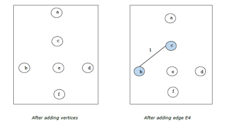
Step-2:

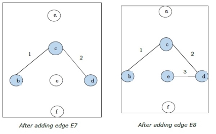
Step-3:

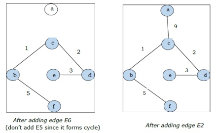
As all the edges are covered in the last figure, the algorithm is stopped and this is considered as the minimal spanning tree and the total weight of the spanning tree is (1+2+3+5+9)=20.

PRIM’S ALGORITHM:

The minimum spanning tree for a connected weighted graph by Prim’s algorithm, developed by the mathematicians VojtechJarnik and Robert C. Prim. In the Graph, the tree that includes every vertex and total weight of all the edges in the tree is less than or equal to every possible spanning tree. Prim’s algorithm works faster on dense graphs.

Algorithm:

Example 2:For instance, consider the following graph G and identify the minimum spanning tree using Prim’s algorithm

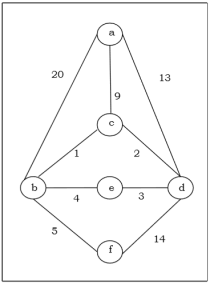
Solution:

It is started with vertex ‘a’.

Step-1:

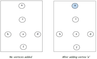
Step-2:

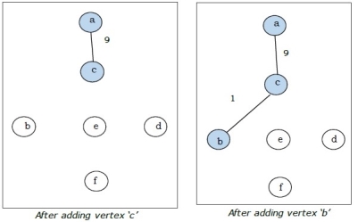
Step-3:

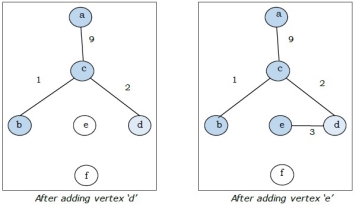
Step-4:

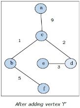
The above graph is the minimum spanning tree and the total weight is

(1+2+3+5+9)=20

5.9 The max-flow-min cut theorem (Transport network)

Statement:

To every weighted s-t graph we can associate a corresponding flow network in which if and otherwise. That is, the edges of the flow network are the same as the edges of the weighted s-t graph, with weights replaced by capacities.

Let f be a maximum flow in a flow network. Consider the set

Consisting of vertices reachable from in the residual network corresponding to . A minimum s-t cut of the corresponding weighted s-t graph is then given by . Furthermore, , that is, the max flow and the cut thus obtained are equal in value.

Lemma 1:

Let be a flow in a flow network . Suppose we have a set such that and . Then the value of the flow equals the total flow leaving S, .

Proof:

(by skew symmetry)

(by flow conservation).

Hence, lemma 1 tells us that we can compute the value of a flow by arbitrarily partitioning the flow network into two sets S and T, where S and  t, and adding only the flows along edges from to T. Intuitively, the conservation of flow implies that the total flow out of  S must equal the total flow emanating from the source; that flow has to get from  S to  T somehow.

LEMMA 2:

Let f be a flow in a flow network . Let C be an s-t cut in the corresponding weighted s-t graph (V, E, s, t, w). Then the value of f,  , is less than or equal to the total weight of C , .

Proof: Since C is an s-t cut, in the weighted s-t graph , there is no path from to t. We can therefore consider the set of all vertices reachable from in this graph. Note that . Applying Lemma 1, we find that.

The idea behind Lemma 2 is simple. The value of a flow, which by Lemma 1 equals the total flow along edges out of S , cannot exceed the total capacity of such edges, but this is precisely the total weight of those edges in the corresponding weighted s-t graph. Lemma 2 is a useful result in its own right, telling us that every flow's value is less than or equal to every cut's weight.

Example: find the minimum flow of the given graph.

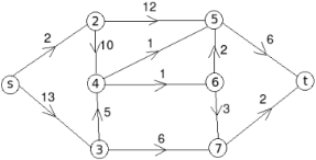
Solution:

Let the edge-labels on the graphs G represent capacity(flow).

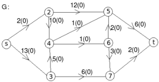
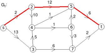
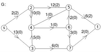
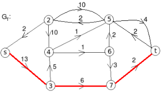
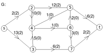
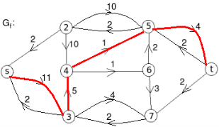
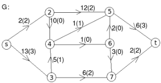
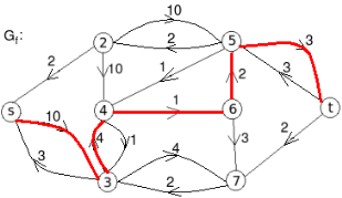
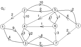
The minimum cut is highlighted in green.

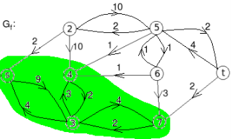
Therefore, the minimum cut has capacity 6 and the maximum flow has flow 6.