2.1 Concept of Sequential Organization | unit 2 linear data structure using sequential organization

FDS

Unit 2

Linear Data Structure using Sequential Organization

2.1 Concept of Sequential Organization

Sequential organization

The physical order during which the records are placed within the file determines the sequence of records.

The relationships among records within the file don't change, except that the file is often extended. There are not any keys. Both the files including database files and files available on device can have sequential organization.

Each record within the file, except the primary, features a unique predecessor record, and every record, except the last, also features a unique successor record.

In data structures, a knowledge structure is claimed to possess sequential access if one can only visit the values it contains in one particular order. The canonical example is that the linked list. Indexing into an inventory that has sequential access requires O(n) time, where n is that the index.

Sequential access is a term defined as a bunch of elements (such as data during a memory array or a computer file or on magnetic tape data storage) being accessed during a predetermined, ordered sequence.

It’s the other of random access, the power to access an arbitrary element of a sequence as easily and efficiently as the other at any time.

Sequential access is usually the sole way of accessing the info , for instance if it's on a tape

It’s going to even be the access method of choice, for instance if all that's wanted is to process a sequence of knowledge elements.

As a result of sequential access, many sorting and searching algorithms like quicksort and binary search may degenerate into bad algorithms that are even less efficient than their naive alternatives; these algorithms are impractical without random access.

The write and skim of records during a physical instead of a logical sequence.

On the opposite hand, some algorithms, typically people who don't have index, require only sequential access, like mergesort, and face no penalty.

2.2 Overview of Array

Array

Element: Every item stored in an array is termed as a component

Index: each memory location of a component in an array is denoted by a numerical index which is used for identifying the element

The array could also be a fixed-size sequenced collection of variables belonging to the same data types. The array has adjacent memory locations to store values. Since the array provides a convenient structure for representing data, it falls under the category of the data structures in C.

The syntax for declaring array are:

Data_typearray_name [array_size];

• An array may be a container of elements.

• Elements have a selected value and data type, like "ABC", TRUE or FALSE, etc.

• Each element also has its own index, which is employed to access the element.

• Elements are stored at contiguous memory locations.

• An index is usually but the entire number of array items.

• In terms of syntax, any variable that's declared as an array can store multiple values.

• Most languages have an equivalent comprehension of arrays but have alternative ways of declaring and initializing them.

Three parts will always remain common altogether the initializations, i.e., array name, elements, and thus the info kind of elements.

• Array name: necessary for straightforward regard to the gathering of elements

• Data Type: necessary for type checking and data integrity

• Elements: these are the info values present in an array

Why can we need arrays?

Here, are some reasons for using arrays:

Arrays are best for storing multiple values during a single variable
Arrays are better at processing many values easily and quickly
Sorting and searching the values is simpler in arrays

2.3 Array as an Abstract Data Type

Arrays are defined as ADT’s because they're capable of holding contiguous elements within the same order. And that they permitaccess for the precise element via index or position.

They are abstract because they will be String, int or Person

int[] arrA = new int[1];

String[] arrB = new String[1];

Person[] arrC = new Person[3]; // where Person is treated as a defined class

Advantages

Fast, random access of things or elements.

Very memory efficient, little or no memory is required aside from that needed to store the contents.

Disadvantages

Slow insertion and deletion of elements

Array size must be known when the array is made and is fixed (static)

2.4 Operations on Array

Basic operations in array

There is some specific operation which can be performed or people that are supported by the array. These are:

Traversing: It prints all the array elements one after another.

Inserting: It adds a component at given index.

Deleting: it's wont to delete a component at given index.

Searching: It searches for an element(s) using given index or by value.

Updating: it's wont to update a component at given index

Array representation

Array can be represented as

int array[10]={10,20,11,30,40,39,23,12,34,16};

• int represents data type

• array represents name of array

• [10] indicates size of array

• {------} inside this parenthesis there are elements of array

elements

index 0 1 2 3 4 5 6 7 8 9

• For an array

• Index always start with 0

• Array length is 10 so it can store 10 elements

• Each element can be accessed with its index.

• Like an element at index 5 is 39.

Size of data types may differ for different data types in array

S no	Data type	Size (default value)
1	bool	False
2	char	0
3	int	0
4	float	0
5	double	0.0f
6	void
7	wchar_t	0

Traversing – this function is to traversing through the elements of array.

2. Inserting- Insert operation is used to insert one or more data elements into an array. Based on thenecessary requirement, a new element can be added at the beginning, end, or any given index of array.

3. Deleting -Deletion refers to removing an existing element from the array and re-organizing all elements of an array.

• Algorithm: - Consider LA is a linear array with N elements and K is a positive integer such that K<=N. Following is the algorithm to delete an element available at the Kth position of LA.

Start

Set J = K

Repeat steps 4 and 5 while J < N

Set LA[J] = LA[J + 1]

Set J = J+1

Set N = N-1

Stop

4. Searching- search operation is used to perform a search for an array element based on its value or its index.

• Algorithm: - Consider LA is a linear array with N elements and K is a positive integer such that K<=N. Following is the algorithm to find an element with a value of ITEM using sequential search

Start

Set J = 0

Repeat steps 4 and 5 while J < N

IF LA[J] is equal ITEM THEN GOTO STEP 6

Set J = J +1

PRINT J, ITEM

Stop

5. Updating - Update operation refers to updating an existing element from the array at a given index.

• Algorithm: -Consider LA is a linear array with N elements and K is a positive integer such that K<=N. Following is the algorithm to update an element available at the Kth position of LA.

Start

Set LA[K-1] = ITEM

Stop

2.5 Merging of two arrays

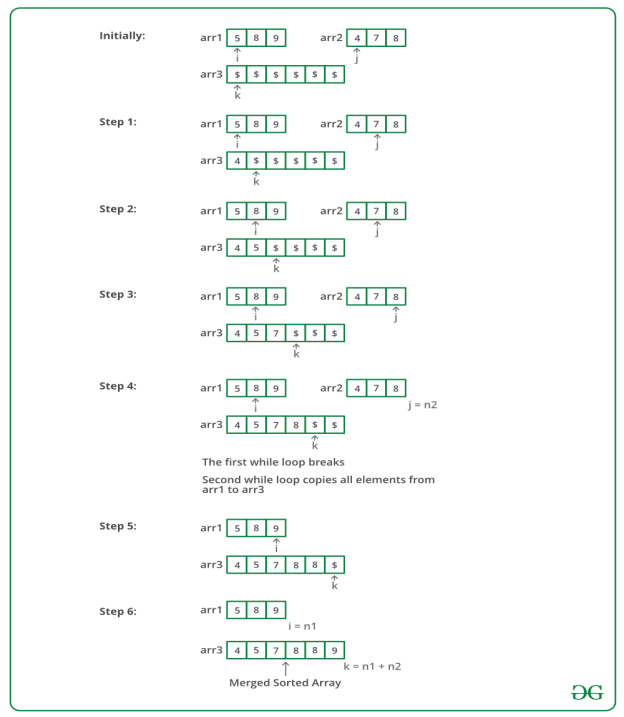
Input: arr1 [] = { 1, 3, 4, 5}, arr2[] = {2, 4, 6, 8}

Output: arr3 [] = {1, 2, 3, 4, 4, 5, 6, 8}

Input: arr1 [] = { 5, 8, 9}, arr2[] = {4, 7, 8}

Output: arr3 [] = {4, 5, 7, 8, 8, 9}

Method 1

• Create an array arr3[] of size n1 + n2.

• Copy all n1 elements of arr1[] to arr3[]

• Traverse arr2[] and one by one insert elements (like insertion sort) of arr3[] to arr1[]. This step take O(n1 * n2) time.

• Time complexity O(n1 * n2)

• Space complexity O(1)

Method 2

• The idea is to use Merge function of Merge sort.

• Create an array arr3[] of size n1 + n2.

• Simultaneously traverse arr1[] and arr2[].

• Pick smaller of current elements in arr1[] and arr2[], copy this smaller element to next position in arr3[] and move ahead in arr3[] and the array whose element is picked.

• If there are remaining elements in arr1[] or arr2[], copy them also in arr3[].

• Time complexity O(n1 + n2)

• Space complexity O(n1 + n2)

Time Complexity: O(n1 + n2)

Auxiliary Space: O(n1 + n2)

$C:\Users\Kilua Zoldyck\Pictures\arrm s.png$

2.6 Advantages and Disadvantages of Arrays

Advantages and drawbacks of Arrays

Advantages

Reading /parsing an array element is simple and efficient. As shown within the above table, the read time of array is O(1) in both best and worst cases. This is often because any element are often instantly read using indexes (base address calculation behind the scene) without traversing the whole array.

Array could also be a foundation of other data structures. For instance other data structures like LinkedList, Stack, Queue etc. are implemented using array.

All the weather of an array are often accessed employing one name (array name) in conjunction with the index, which is readable, user-friendly and efficient rather than storing those elements in different-2 variables.

Disadvantages

While using array, we must need to make the selection of the size of the array within the start, so if we aren't aware what percentage elements we are becoming to store in array, it'd make the task difficult.

The size of the array is fixed so if at later point; if we'd wish to store more elements in it then it can’t be done. On the other hand, if we store less number of elements than the declared size, the remaining allocated memory is wasted.

2.7 Storage Representation and their Address Calculation: Row major and Column Major

One Dimensional Array

• Simplest arrangement that creates use of computed address to locate its elements is that the one dimensional array or vector; number of memory locations is sequentially allocated to the vector

• A vector size is fixed and thus requires a hard and fast number of memory locations.

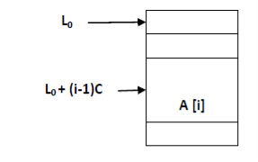
• Vector A with subscript boundary of “one” is represented as below….

• L0 is that the address of the primary word allocated to the primary element of vector A.

• C words are allocated for every element or node

• For a given equation the address of A is Loc (Ai) = L0 + C (i-1)

• Let’s consider the more general case of representing a vector A whose boundary for its subscript is given by some variable b.

• For a given equation the location of A is Loc (Ai) = L0 + C (i-b)

$C:\Users\Kilua Zoldyck\Pictures\a.png$

An array can be stored in many ways

Array A= [ a11 a12 a13 ]

[ a21 a22 a23 ]

Array could be stored in possible ways

Index	Row major	Column major
0	A11	A11
1	A12	A21
2	A13	A12
3	A21	A22
4	A22	A13
5	A23	A23

Different programming languages handles array in different ways.

• In C programming , multidimensional arrays are stored in row-major order, and the array indexes are written row-first (lexicographical access order):

C: row-major order (lexicographical access order), zero-based indexing

Index	Value	Access
0	A11	A[0][0]
1	A12	A[0][1]
2	A13	A[0][2]
3	A21	A[1][0]
4	A22	A[1][1]
5	A23	A[1][2]

• Address of [I, J]th element in row-major = B + W[C(I – Kr) + (J – Kc)]

• In Fortran, arrays are stored in column-major order, while the array indexes are still written row-first (colexico graphical access order):

Fortran: column-major order (colexographical access order), one-based indexing

Index	Value	Access
1	A11	A[1][1]
2	A21	A[2][1]
3	A12	A[1][2]
4	A22	A[2][2]
5	A13	A[1][3]
6	A23	A[2][3]

• Address of [I, J]th element in column-major = B + W[R(J – Kc) + (I – Kr)]

• Where :

• B is the base address (address of the first block in the array).

• W is the width in bytes (size in bytes for each block in the array).

• Kr is the index of the first row.

• Kc is the index of the first column.

• R is the total number of rows.

• C is the total number of columns.

2.8 Multidimensional Arrays: Two-dimensional arrays, n-dimensional arrays.

Two Dimensional Array

• Two dimensional arrays also are called table or matrix, two dimensional arrays have two subscripts

• Two dimensional array during which elements are stored column by column is named as column major matrix

• Two dimensional array during which elements are stored row by row is named as row major matrix

• First subscript denotes number of rows and second subscript denotes the amount of columns

• Two dimensional array consisting of two rows and 4 columns as above Fig is stored sequentially by columns : A [ 1, 1 ], A [ 2 , 1 ], A [ 1 , 2 ], A [ 2 , 2 ], A [ 1 , 3 ], A [ 2 , 3 ], A [ 1, 4 ], A [ 2, 4 ]

• The address of element A [ i , j ] are often obtained by expression Loc (A [ i , j ]) = L0 + (j-1)*2 + i-1 generally for 2 dimensional array consisting of n rows and m columns the address element A [ i, j ] is given by Loc (A [ i , j ]) = L0 + (j-1)*n + (i – 1)

• In row major matrix, array are often generalized to arbitrary lower and boundary in its subscripts, assume that b1 ≤ I ≤ u1 and b2 ≤ j ≤u2

For row major matrix: Loc (A [ i , j ]) = L0 + ( i – b1 ) *(u2-b2+1) + (j-b2)

Applications of Array

Symbol Manipulation (matrix representation of polynomial equation)

Sparse Matrix

2.9 Concept of Ordered List

Ordered list

• The structure of an ordered list is a collection of items where each item holds a relative position that is based upon some underlying characteristic of the item.

• The ordering is typically either ascending or descending and we assume that list items have a meaningful comparison operation that is already defined.

• Many of the ordered list operations are the same as those of the unordered list.

• OrderedList() creates a new empty ordered list. It doesn’t require any parameters and returns an empty list.

• add(item) adds a new item to the list making sure that the order is preserved. It needs the item and returns nothing. Assume the item is not already in the list.

• remove(item) removes the item from the list. It needs the item and modifies the list. Assume the item is present in the list.

• search(item) searches for the item in the list. It needs the item and returns a boolean value.

• isEmpty() tests to see whether the list is empty. It needs no parameters and returns a boolean value.

• size() returns the number of items in the list. It needs no parameters and returns an integer.

• index(item) returns the position of item in the list. It needs the item and returns the index. Assume the item is in the list.

• pop() removes and returns the last item in the list. It needs nothing and returns an item. Assume the list has at least one item.

• pop(pos) removes and returns the item at position pos. It needs the position and returns the item. Assume the item is in the list.

Array and ordered list

S no	Array	Ordered list
1	An array is a contiguous segment of memory, and a list is just a bunch of nodes, each one has the pointers to the "next" node (and also to the "previous" node, in the case of bidirectional lists).	The structure of an ordered list is a collection of items where each item holds a relative position that is based upon some underlying characteristic of the item. The ordering is typically either ascending or descending and we assume that list items have a meaningful comparison operation that is already defined.
2	Arrays efficiently - in O(1) - support random access (i.e. by arbitrary given index i),	Lists, on the other hand, do not support efficient random access (while supporting efficient consecutive traversal)
3	Deleting/inserting an element into an array is slow - O(n), because you have to move all elements after deleting/inserting element	Inserting and deleting is fast - O(1).
4	In the array, you have to shuffle other entries around; in a list, you simply adjust appropriate pointers in at most 3 elements	it is possible to add items to a particular point in the list more swiftly than it is possible to add a new item in an array at an equivalent point
5	Access to the Nth item takeO(1) time for an array.	Access to the Nth item in a list takes O(N) time
6	The items in an array are not necessarily in any particular order	The items in a list are always arranged in any particular order
7	With arrays, you can do random access of a member in O(1), while this takes O(N) in an list.	Performance wise, maintaining an ordered list is pretty expensive: O(N) insert, delete, but you can do searches faster than O(N) (using something like binary search)

2.10 Single Variable Polynomial: Representation using arrays, Polynomial as array of structure, Polynomial addition, Polynomial multiplication.

Symbol Manipulation using Array

• We will use array for various quite operations in polynomial equation like addition, subtraction, division, differentiation etc…

• We have an interest find suitable representation for polynomial in order that different operations like addition, subtraction etc… are often performed in efficient manner

• Array are often used to represent Polynomial equation

• Matrix Representation of Polynomial equation

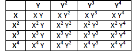
$C:\Users\Kilua Zoldyck\Pictures\xs.png$

$C:\Users\Kilua Zoldyck\Pictures\aw.png$

• Once we've algorithm for converting the polynomial equation to an array representation and another algorithm for converting array to polynomial equation, then different operations in array (matrix) are going to be corresponding operations of polynomial equation

Storing of polynomial in an array

Eg :- for a polynomial p1= 5x6 +10x3 -11x2 +12x+18

Representing power of x	0	1	2	3	4	5	6	7
Element	18	12	-11	10	0	0	5	0
index	0	1	2	3	4	5	6	7

Array will be represented as A={18, 12,-11,10,0,0,5}

• the coefficient 18 is in slot 0 of the array (representing 18x^0)

• the coefficient 12 is in slot 1 of the array (representing 12x^1)

• the coefficient -11 is in slot 2 of the array (representing11x^2)

• the coefficient 10 is in slot 3 of the array (representing 10x^3)

• the coefficient 5 is in slot 6 of the array (representing 5x^6)

Advantage

Only good for non-sparse polynomials

Ease of storage and retrieval

Disadvantage

• Have to allocate size ahead of time

• Huge array size required for sparse polynomials waste of space and runtime.

• This polynomial representation in array is not good for higher degrees of polynomial .

• Array representation cost too much memory to be wasted for higher degree of polynomial

• Will consume too much time for searching element and wasting too much memory that used for allocation .]

• Foreg. for a polynomial like p=5x34 +15x19 +10x13 -11x8 +12x4+18

• Or for higher degree polynomial 50x6000 +100x3000 -141x200 +112x+18

For a polynomial p=6x50 +10x3 -11x2 +12x+18

• polynomial = new array(50) // I'm assuming all elements initialize to zero

• polynomial[50] = 6

• polynomial[3] = 10

• polynomial[2] = -11

• polynomial[1] = 12

• polynomial[0] = 18

The basic idea of polynomial addition is to add coefficient parts of the polynomials having same exponent.

Polynomial addition

A polynomial is an expression that contains quite two terms. A term is formed from coefficient and exponent.

Example: P(x) = 4x3+6x2+7x+9

A polynomial could also be represented using array or structure. A structure could also be defined such it contains two parts – one is that the coefficient and second is that the corresponding exponent. The structure definition could also be given as shown below:

Structpolynomial{

int coefficient;

int exponent;

};

Algorithm: adding polynomial using structures

AddPoly(Struct Poly p1[10], Struct Poly p2[10], int t1,int t2,Struct Poly p3[10])

[Initialize segment variables]

[Initialize Counter] Set i=0,j=0,k=0

2. Repeat step 3 while i<t1 and j<t2

If p1[i].expo=p2[j].expo, then

3. p3[i].coeff=p1[i].coeff+p2[i].coeff

p3[k].expo=p1[i].expo

[Increase counter] Set i=i+1,j=j+1,k=k+1

else if p1[i].expo > p2[j].expo, then

p3[k].coeff=p1[i].coeff

p3[k].expo=p1[i].expo

[Increase counter] Set i=i+1,k=k+1

else

p3[k].coeff=p2[j].coeff

p3[k].expo=p2[j].expo

Set j=j+1,k=k+1

[End of If]

[End of loop]

4. Repeat while i<t1

p3[k].coeff=p1[i].coeff

p3[k].expo=p1[i].expo

Set i=i+1,k=k+1

[End of loop]

5. Repeat while j<t2

p3[k].coeff=p2[j].coeff

p3[k].expo=p2[j].expo

Set j=j+1,k=k+1

[End of loop]

6. Return k

7. Exit

Adding polynomial using array

Addition of polynomial is easy as compared to multiplication

add (A[0..m-1], B[0..n01])

1) Create a sum array sum[] of size equal to maximum of 'm' and 'n'

2) Copy A[] to sum[].

3) Traverse array B[] and do following for every element B[i]

4) sum[i] = sum[i] + B[i]

5) Return sum[].

Example:

Input: A [] = {5, 0, 10, 6} similar to Pa =6x3+10x2+5

B [] = {1, 2, 4} similar to Pb =4x2+2x+1

Output: sum [] = {6, 2, 14, 6} similar to Psum= 6x3+14x2+2x+6

Example 2

P1=1x3+5x2+3x+2

P2=5x2+8x+7

Padd=1x3+10x2+11x+9

Enter the highest degree of polynomial 1 = 3

Enter the coeff of x^0 =2

Enter the coeff of x^1 =3

Enter the coeff of x^2 =5

Enter the coeff of x^3=1

Enter the highest degree of polynomial2=2

Enter the coeff of x^0 =7

Enter the coeff of x^1 =8

Enter the coeff of x^2 =5

Expression 1 = 2.0+ 3.0x^1+ 5.0x^2+ 1.0x^3

Expression 2 = 7.0+ 8.0x^1+ 5.0x^2

Expression after addition = 9.0+ 11.0x^1+ 10.0x^2+ 1.0x^3

Time complexity

Time complexity of adding two polynomial O(m+n)

where m and n are orders of two given polynomials.

Multiplication of Two Polynomial

Multiplication of two polynomials however requires manipulation of each node such that the exponents are added up and the coefficients are multiplied. After each term of first polynomial is operated upon with each term of the second polynomial, then the result has to be added up by comparing the exponents and adding the coefficients for similar exponents and including terms as such with dissimilar exponents in the result

Algorithm:

multiply(A[0..m-1], B[0..n01])

1) Create a product array prod[] of size m+n-1.

2) Initialize all entries in prod[] as 0

3) Traverse array A[] and do following for every element A[i]

Traverse array B[] and do following for every element B[j]

prod[i+j] = prod[i+j] + A[i] * B[j]

4) Return prod[].

A simple solution is to one by one consider every term of first polynomial and multiply it with every term of second polynomial.

Example:-

Input: A [] = {5, 0, 10, 6} similar to Pa =6x3+10x2+5

B [] = {1, 2, 4} similar to Pb =4x2+2x+1

Output: prod [] = {5, 10, 30, 26, 52, 24}

Similar toPmul= 24x5+52x4+26x3+30x2+10x+5

p1=4x2+3x+2

p2=2x3+7x2+6x+5

pmul= 2x3+28x2+18x+10

Enter the highest degree of polynomial1= 2

Enter the coeff of x^0 = 2

Enter the coeff of x^1 = 3

Enter thecoeff of x^2 =4

Enter the highest degree of polynomial 2 = 3

Enter the coeff of x^0 = 5

Enter the coeff of x^1 = 6

Enter the coeff of x^2 = 7

Enter the coeff of x^3 = 2

Expression 1 = 2.0+ 3.0x^1+ 4.0x^2

Expression 2 = 5.0+ 6.0x^1+ 7.0x^2+ 2.0x^3

Expression after multiplication = 10.0+ 18.0x^1+ 28.0x^2+ 2.0x^3

2.11 Sparse Matrix: Sparse matrix representation using array, Sparse matrix addition, Transpose of sparse matrix- Simple and Fast Transpose, Time and Space tradeoff

Sparse matrix

Sparse matrix is amatrix in which most of the elements are zero

• An mXn matrix is claimed to be sparse if “many” of its elements are zero.

• By contrast if most of the elements are non zero then the matrix is considered as ‘dense’ .

• Sparcity of a sparse matrix is the number of zero valued element divided by total number of elements

• We can device a simple representation scheme whose space requirement equals the size of the nonzero elements.

Example:-

• The non-zero entries of a sparse matrix could also be mapped into a linear list in row-major order.

• for instance the non-zero entries of 4X8 matrix of below

• in row major order are 2, 1, 6, 7,3, 9, 8, 4, 5

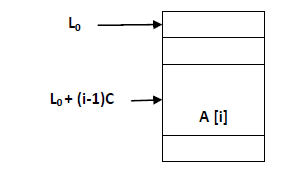
Figure A 4 x 4 matrix

Figure, Linear Representation of above matrix

• To construct matrix structure we need to record

(a) Original row and columns of every non zero entries

(b) No of rows and columns within the matrix

• So each element of the array into which the sparse matrix is mapped need to have three fields: row, column and value

• A corresponding amount of time is saved creating the linear list representation over initialization of two dimension array.

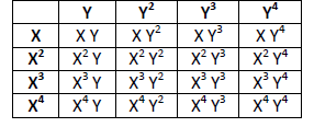
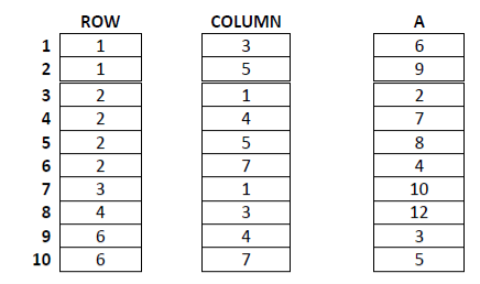
• Here from 6X7=42 elements, only 10 are non zero. A[1,3]=6, A[1,5]=9, A[2,1]=2, A[2,4]=7, A[2,5]=8, A[2,7]=4, A[3,1]=10, A[4,3]=12, A[6,4]=3, A[6,7]=5.

• One basic method for storing such a sparse matrix is to store non-zero elements in one dimensional array and to spot each array elements with row and column indices

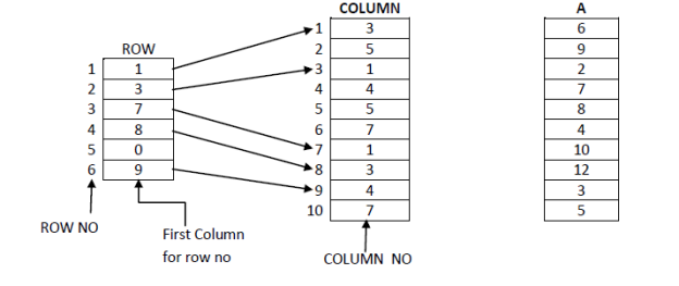
$C:\Users\Kilua Zoldyck\Pictures\aq.png$

$C:\Users\Kilua Zoldyck\Pictures\aqwe.png$

• A more efficient representation in terms of storage requirement and access time to the row of the matrix is shown in fid (d). The row vector changed in order that its ith element is that the index to the primary of the column indices for the element in row I of the matrix.

Linked Representation of Sparse matrix

Typical node to represent non-zero element is

$C:\Users\Kilua Zoldyck\Pictures\spm.png$

Figure:-linked representation of sparse matrix

Transpose of sparse matrix

To Transpose a matrix, we will simply change every column value to the row value and vice-versa,

However, during this case, the resultant matrix won’t be sorted as we require.

Hence, we initially determine the number of elements less than the current element’s column being inserted in order to get the exact index of the resultant matrix where the current element should be placed.

This is done by maintaining an array index[] whose ith value indicates the number of elements in the matrix less than the column i.

Algorithm for Transpose of Sparse Matrix

SparseMatrixSparseMatrix::Transpose()

{

Construct a SparseMatrix, b(cols, rows, terms);
If (terms > 0)

{

Let rowSize be an integer array of size cols.
Let rowStart be an integer array of size cols.
Initialize each element in rowSize to 0.
For (i=0; i
rowSize [smArray[i].col]++;
rowStart [0] = 0;
For (i = 1; i< cols; i++)
rowStart [i] = rowSize [i-1] + rowStart [i-1];
For (i=0; i< terms; i++) {
j = rowStart [ smArray [i].col ];
Copy smArray[ i ] to smArray[ j ];
Interchange row and col of smArray[ j ];
rowStart [ smArray [i].col ]++;

}
}
Return b;
}

Multiplication of sparse matrix

To Multiply the matrices, we first calculate transpose of the second matrix to simplify our comparisons and maintain the sorted order.

So, the resultant matrix is obtained by traversing through the whole length of both matrices and summing the acceptable multiplied values.

Any row value adequate to x within the first matrix and row value adequate to y within the second matrix (transposed one) will contribute towards result[x][y].

This is obtained by multiplying all such elements having col value in both matrices and adding only those with the row as x in first matrix and row as y within the second transposed matrix to urge the result[x][y].

Multiplying Sparse Matrices

1 void mm_mul_sa (sa_t *A, sa_t *B, sa_t *C)

2 {

3 inti, j, k;

4 int sum;

6 for (i = 0; i< A->num_rows; i++) {

7 for (j = 0; j < B->num_cols; j++) {

8 sum = 0;

9 for (k = 0; k < A->num_cols; k++) {

10 sum += saGet (A,i,k) * saGet (B,k,j);

11 }

12 saSet (C,i,j,sum);

13 }

14 }

15 }

Row Col Val Row Col Val

1 2 10 1 1 2

1 3 12 1 2 5

2 1 1 2 2 1

2 3 2 3 1 8

The resulting matrix after multiplication will be obtained as follows:

Transpose of second matrix:

Row Col Val Row Col Val

1 2 10 1 1 2

1 3 12 1 3 8

2 1 1 2 1 5

2 3 2 2 2 1

Summation of multiplied values:

result[1][1] = A[1][3]*B[1][3] = 12*8 = 96

result[1][2] = A[1][2]*B[2][2] = 10*1 = 10

result[2][1] = A[2][1]*B[1][1] + A[2][3]*B[1][3] = 2*1 + 2*8 = 18

result[2][2] = A[2][1]*B[2][1] = 1*5 = 5

Any other element cannot be obtained by any combination of row in

Matrix A and Row in Matrix B.

Hence the final resultant matrix will be:

Row Col Val

1 1 96

1 2 10

2 1 18

Matrix operations

Matrix 1: (4x4)

Row ColumnValue

1 2 10

1 4 12

3 3 5

4 1 15

4 2 12

Matrix 2: (4X4)

Row Column Value

1 3 8

2 4 23

3 3 9

4 1 20

4 2 25

Output:

Result of Addition: (4x4)

Row Column Value

1 2 10

1 3 8

1 4 12

2 4 23

3 3 14

4 1 35

4 2 37

Result of Multiplication: (4x4)

Row Column Value

1 1 240

1 2 300

1 4 230

3 3 45

4 3 120

4 4 276

Result of transpose on the first matrix: (4x4)

Row Column Value

1 4 15

2 1 10

2 4 12

3 3 5

4 1 1

Time Complexity

Addition operation of sparse matrix has time complexity of, hence, has a time complexity of O(n),

Addition operation traverses the matrices linearly
where n is the number of non-zero elements in the larger matrix amongst the two.

Transpose of sparse matrix has a time complexity of O(n+m)

Where n is the number of columns and m is the number of non-zero elements in the matrix

During worst case when matrix is not a sparse matrix T(n)=O(m^2*n),

where 'm' is the length of the first array and
'n' is the length of the second array and with the optimization,
We can reduce it by a constant K where K is the no of zero's in the matrix A.

Multiplication of sparse matrix has a time complexity of O(x*n + y*m),

where (x, m) is number of columns and terms in the second matrix;
and (y, n) is number of rows and terms in the first matrix.

Sign Up

Index

Notes

Highlighted

Underlined

Browse by Topics

Notes

Highlighted

Underlined