Hashing
Hash Table is a data structure which stores data in an associative manner. In a hash table, data is stored in an array format, where each data value has its own unique index value. Access of data becomes very fast if we know the index of the desired data.
Thus, it becomes a data structure in which insertion and search operations are very fast irrespective of the size of the data. Hash Table uses an array as a storage medium and uses hash technique to generate an index where an element is to be inserted or is to be located from.
Hashing
Hashing is a technique to convert a range of key values into a range of indexes of an array. We're going to use modulo operator to get a range of key values. Consider an example of hash table of size 20, and the following items are to be stored. Item are in the (key, value) format.

Fig1- Hash function
Sr. No. | Key | Hash | Array Index |
1 | 1 | 1 % 20 = 1 | 1 |
2 | 2 | 2 % 20 = 2 | 2 |
3 | 42 | 42 % 20 = 2 | 2 |
4 | 4 | 4 % 20 = 4 | 4 |
5 | 12 | 12 % 20 = 12 | 12 |
6 | 14 | 14 % 20 = 14 | 14 |
7 | 17 | 17 % 20 = 17 | 17 |
8 | 13 | 13 % 20 = 13 | 13 |
9 | 37 | 37 % 20 = 17 | 17 |
Linear Probing
As we can see, it may happen that the hashing technique is used to create an already used index of the array. In such a case, we can search the next empty location in the array by looking into the next cell until we find an empty cell. This technique is called linear probing.
Sr. No. | Key | Hash | Array Index | After Linear Probing, Array Index |
1 | 1 | 1 % 20 = 1 | 1 | 1 |
2 | 2 | 2 % 20 = 2 | 2 | 2 |
3 | 42 | 42 % 20 = 2 | 2 | 3 |
4 | 4 | 4 % 20 = 4 | 4 | 4 |
5 | 12 | 12 % 20 = 12 | 12 | 12 |
6 | 14 | 14 % 20 = 14 | 14 | 14 |
7 | 17 | 17 % 20 = 17 | 17 | 17 |
8 | 13 | 13 % 20 = 13 | 13 | 13 |
9 | 37 | 37 % 20 = 17 | 17 | 18 |
Basic Operations
Following are the basic primary operations of a hash table.
DataItem
Define a data item having some data and key, based on which the search is to be conducted in a hash table.
struct DataItem {
int data;
int key;
};
Hash Method
Define a hashing method to compute the hash code of the key of the data item.
int hashCode(int key){
return key % SIZE;
}
Search Operation
Whenever an element is to be searched, compute the hash code of the key passed and locate the element using that hash code as index in the array. Use linear probing to get the element ahead if the element is not found at the computed hash code.
Example
struct DataItem *search(int key) {
//get the hash
int hashIndex = hashCode(key);
//move in array until an empty
while(hashArray[hashIndex] != NULL) {
if(hashArray[hashIndex]->key == key)
return hashArray[hashIndex];
//go to next cell
++hashIndex;
//wrap around the table
hashIndex %= SIZE;
}
return NULL;
}
Insert Operation
Whenever an element is to be inserted, compute the hash code of the key passed and locate the index using that hash code as an index in the array. Use linear probing for empty location, if an element is found at the computed hash code.
Example
void insert(int key,int data) {
struct DataItem *item = (struct DataItem*) malloc(sizeof(struct DataItem));
item->data = data;
item->key = key;
//get the hash
int hashIndex = hashCode(key);
//move in array until an empty or deleted cell
while(hashArray[hashIndex] != NULL && hashArray[hashIndex]->key != -1) {
//go to next cell
++hashIndex;
//wrap around the table
hashIndex %= SIZE;
}
hashArray[hashIndex] = item;
}
Delete Operation
Whenever an element is to be deleted, compute the hash code of the key passed and locate the index using that hash code as an index in the array. Use linear probing to get the element ahead if an element is not found at the computed hash code. When found, store a dummy item there to keep the performance of the hash table intact.
Example
struct DataItem* delete(struct DataItem* item) {
int key = item->key;
//get the hash
int hashIndex = hashCode(key);
//move in array until an empty
while(hashArray[hashIndex] !=NULL) {
if(hashArray[hashIndex]->key == key) {
struct DataItem* temp = hashArray[hashIndex];
//assign a dummy item at deleted position
hashArray[hashIndex] = dummyItem;
return temp;
}
//go to next cell
++hashIndex;
//wrap around the table
hashIndex %= SIZE;
}
return NULL;
}
Hash Table Program in C
Hash Table is a data structure which stores data in an associative manner. In hash table, the data is stored in an array format where each data value has its own unique index value. Access of data becomes very fast, if we know the index of the desired data.
Implementation in C
#include <stdio.h>
#include <string.h>
#include <stdlib.h>
#include <stdbool.h>
#define SIZE 20
struct DataItem {
int data;
int key;
};
struct DataItem* hashArray[SIZE];
struct DataItem* dummyItem;
struct DataItem* item;
int hashCode(int key) {
return key % SIZE;
}
struct DataItem *search(int key) {
//get the hash
int hashIndex = hashCode(key);
//move in array until an empty
while(hashArray[hashIndex] != NULL) {
if(hashArray[hashIndex]->key == key)
return hashArray[hashIndex];
//go to next cell
++hashIndex;
//wrap around the table
hashIndex %= SIZE;
}
return NULL;
}
void insert(int key,int data) {
struct DataItem *item = (struct DataItem*) malloc(sizeof(struct DataItem));
item->data = data;
item->key = key;
//get the hash
int hashIndex = hashCode(key);
//move in array until an empty or deleted cell
while(hashArray[hashIndex] != NULL && hashArray[hashIndex]->key != -1) {
//go to next cell
++hashIndex;
//wrap around the table
hashIndex %= SIZE;
}
hashArray[hashIndex] = item;
}
struct DataItem* delete(struct DataItem* item) {
int key = item->key;
//get the hash
int hashIndex = hashCode(key);
//move in array until an empty
while(hashArray[hashIndex] != NULL) {
if(hashArray[hashIndex]->key == key) {
struct DataItem* temp = hashArray[hashIndex];
//assign a dummy item at deleted position
hashArray[hashIndex] = dummyItem;
return temp;
}
//go to next cell
++hashIndex;
//wrap around the table
hashIndex %= SIZE;
}
return NULL;
}
void display() {
int i = 0;
for(i = 0; i<SIZE; i++) {
if(hashArray[i] != NULL)
printf(" (%d,%d)",hashArray[i]->key,hashArray[i]->data);
else
printf(" ~~ ");
}
printf("\n");
}
int main() {
dummyItem = (struct DataItem*) malloc(sizeof(struct DataItem));
dummyItem->data = -1;
dummyItem->key = -1;
insert(1, 20);
insert(2, 70);
insert(42, 80);
insert(4, 25);
insert(12, 44);
insert(14, 32);
insert(17, 11);
insert(13, 78);
insert(37, 97);
display();
item = search(37);
if(item != NULL) {
printf("Element found: %d\n", item->data);
} else {
printf("Element not found\n");
}
delete(item);
item = search(37);
if(item != NULL) {
printf("Element found: %d\n", item->data);
} else {
printf("Element not found\n");
}
}
If we compile and run the above program, it will produce the following result −
Output
~~ (1,20) (2,70) (42,80) (4,25) ~~ ~~ ~~ ~~ ~~ ~~ ~~ (12,44) (13,78) (14,32) ~~ ~~ (17,11) (37,97) ~~
Element found: 97
Element not found
Key takeaway
Hash Table is a data structure which stores data in an associative manner. In a hash table, data is stored in an array format, where each data value has its own unique index value. Access of data becomes very fast if we know the index of the desired data.
Thus, it becomes a data structure in which insertion and search operations are very fast irrespective of the size of the data. Hash Table uses an array as a storage medium and uses hash technique to generate an index where an element is to be inserted or is to be located from.
What is Hashing?
What is Hash Function?
What is Hash Table?

Fig 2 – Hash table
Hash Key = Key Value % Number of Slots in the Table
Data Item | Value % No. of Slots | Hash Value |
26 | 26 % 10 = 6 | 6 |
70 | 70 % 10 = 0 | 0 |
18 | 18 % 10 = 8 | 8 |
31 | 31 % 10 = 1 | 1 |
54 | 54 % 10 = 4 | 4 |
93 | 93 % 10 = 3 | 3 |

Linear Probing
P = (1 + P) % (MOD) Table_size
For example,

If we insert next item 40 in our collection, it would have a hash value of 0 (40 % 10 = 0). But 70 also had a hash value of 0, it becomes a problem.
Linear probing solves this problem:
P = H(40)
44 % 10 = 0
Position 0 is occupied by 70. so we look elsewhere for a position to store 40.
Using Linear Probing:
P= (P + 1) % table-size
0 + 1 % 10 = 1
But, position 1 is occupied by 31, so we look elsewhere for a position to store 40.
Using linear probing, we try next position: 1 + 1 % 10 = 2
Position 2 is empty, so 40 is inserted there.

Key takeaway
Following are the basic primary operations of a hash table.
DataItem
Define a data item having some data and key, based on which the search is to be conducted in a hash table.
struct DataItem {
int data;
int key;
};
Hash Method
Define a hashing method to compute the hash code of the key of the data item.
int hashCode(int key){
return key % SIZE;
}
Search Operation
Whenever an element is to be searched, compute the hash code of the key passed and locate the element using that hash code as index in the array. Use linear probing to get the element ahead if the element is not found at the computed hash code.
Example
struct DataItem *search(int key) {
//get the hash
int hashIndex = hashCode(key);
//move in array until an empty
while(hashArray[hashIndex] != NULL) {
if(hashArray[hashIndex]->key == key)
return hashArray[hashIndex];
//go to next cell
++hashIndex;
//wrap around the table
hashIndex %= SIZE;
}
return NULL;
}
Insert Operation
Whenever an element is to be inserted, compute the hash code of the key passed and locate the index using that hash code as an index in the array. Use linear probing for empty location, if an element is found at the computed hash code.
Example
void insert(int key,int data) {
struct DataItem *item = (struct DataItem*) malloc(sizeof(struct DataItem));
item->data = data;
item->key = key;
//get the hash
int hashIndex = hashCode(key);
//move in array until an empty or deleted cell
while(hashArray[hashIndex] != NULL && hashArray[hashIndex]->key != -1) {
//go to next cell
++hashIndex;
//wrap around the table
hashIndex %= SIZE;
}
hashArray[hashIndex] = item;
}
Delete Operation
Whenever an element is to be deleted, compute the hash code of the key passed and locate the index using that hash code as an index in the array. Use linear probing to get the element ahead if an element is not found at the computed hash code. When found, store a dummy item there to keep the performance of the hash table intact.
Example
struct DataItem* delete(struct DataItem* item) {
int key = item->key;
//get the hash
int hashIndex = hashCode(key);
//move in array until an empty
while(hashArray[hashIndex] !=NULL) {
if(hashArray[hashIndex]->key == key) {
struct DataItem* temp = hashArray[hashIndex];
//assign a dummy item at deleted position
hashArray[hashIndex] = dummyItem;
return temp;
}
//go to next cell
++hashIndex;
//wrap around the table
hashIndex %= SIZE;
}
return NULL;
}
In computing, a hash table [hash map] is a data structure that provides virtually direct access to objects based on a key [a unique String or Integer]. A hash table uses a hash function to compute an index into an array of buckets or slots, from which the desired value can be found. Here are the main features of the key used:
Hash buckets are used to apportion data items for sorting or lookup purposes. The aim of this work is to weaken the linked lists so that searching for a specific item can be accessed within a shorter timeframe. 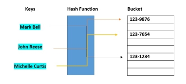
Fig 3 – Hash Bucket
A hash table that uses buckets is actually a combination of an array and a linked list. Each element in the array [the hash table] is a header for a linked list. All elements that hash into the same location will be stored in the list. The hash function assigns each record to the first slot within one of the buckets. In case the slot is occupied, then the bucket slots will be searched sequentially until an open slot is found. In case a bucket is completely full, the record will get stored in an overflow bucket of infinite capacity at the end of the table. All buckets share the same overflow bucket. However, a good implementation will use a hash function that distributes the records evenly among the buckets so that as few records as possible go into the overflow bucket.
1.3.3 What is Collision?
Since a hash function gets us a small number for a key which is a big integer or string, there is a possibility that two keys result in the same value. The situation where a newly inserted key maps to an already occupied slot in the hash table is called collision and must be handled using some collision handling technique.
What are the chances of collisions with large table?
Collisions are very likely even if we have big table to store keys. An important observation is Birthday Paradox. With only 23 persons, the probability that two people have the same birthday is 50%.
How to handle Collisions?
There are mainly two methods to handle collision:
1) Separate Chaining
2) Open Addressing
In this article, only separate chaining is discussed. We will be discussing Open addressing in the next post.
Separate Chaining:
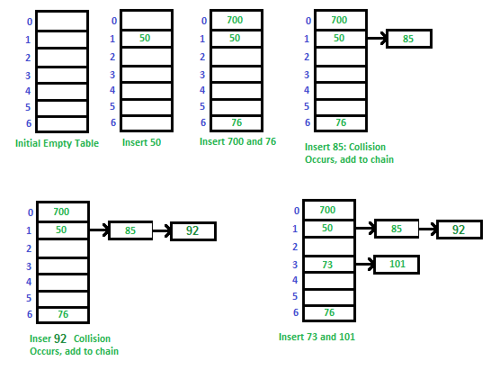
The idea is to make each cell of hash table point to a linked list of records that have same hash function value.
Let us consider a simple hash function as “key mod 7” and sequence of keys as 50, 700, 76, 85, 92, 73, 101.
Fig 4 - Example
Advantages:
1) Simple to implement.
2) Hash table never fills up; we can always add more elements to the chain.
3) Less sensitive to the hash function or load factors.
4) It is mostly used when it is unknown how many and how frequently keys may be inserted or deleted.
Disadvantages:
1) Cache performance of chaining is not good as keys are stored using a linked list. Open addressing provides better cache performance as everything is stored in the same table.
2) Wastage of Space (Some Parts of hash table are never used)
3) If the chain becomes long, then search time can become O(n) in the worst case.
4) Uses extra space for links.
Performance of Chaining:
Performance of hashing can be evaluated under the assumption that each key is equally likely to be hashed to any slot of table (simple uniform hashing).
m = Number of slots in hash table
n = Number of keys to be inserted in hash table
Load factor α = n/m
Expected time to search = O(1 + α)
Expected time to delete = O(1 + α)
Time to insert = O(1)
Time complexity of search insert and delete is
O(1) if α is O(1)
1.3.4 Probing
In this section we will see what is linear probing technique in open addressing scheme. There is an ordinary hash function h´(x): U → {0, 1, . . ., m – 1}. In open addressing scheme, the actual hash function h(x) is taking the ordinary hash function h’(x) and attach some another part with it to make one linear equation.
h´(𝑥) = 𝑥 𝑚𝑜𝑑 𝑚
ℎ(𝑥, 𝑖) = (ℎ´(𝑥) + 𝑖)𝑚𝑜𝑑 𝑚
The value of i| = 0, 1, . . ., m – 1. So we start from i = 0, and increase this until we get one free space. So initially when i = 0, then the h(x, i) is same as h´(x).
Example
Suppose we have a list of size 20 (m = 20). We want to put some elements in linear probing fashion. The elements are {96, 48, 63, 29, 87, 77, 48, 65, 69, 94, 61}
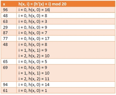
Hash Table

Hashing
We have all used a dictionary, and many of us have a word processor equipped with a limited dictionary, that is a spelling checker. We consider the dictionary, as an ADT. Examples of dictionaries are found in many applications, including the spelling checker, the thesaurus, the data dictionary found in database management applications, and the symbol tables generated by loaders, assemblers, and compilers.
In computer science, we generally use the term symbol table rather than dictionary, when referring to the ADT. Viewed from this perspective, we define the symbol table as a set of name-attribute pairs. The characteristics of the name and attribute vary according to the application. For example, in a thesaurus, the name is a word, and the attribute is a list of synonyms for the word; in a symbol table for a compiler, the name is an identifier, and the attributes might include an initial value and a list of lines that use the identifier.
Generally, we would want to perform the following operations on any symbol table:
(1) Determine if a particular name is in the table
(2) Retrieve the attributes of that name
(3) Modify the attributes of that name
(4) Insert a new name and its attributes
(5) Delete a name and its attributes
There are only three basic operations on symbol tables: searching, inserting, and deleting. The technique for those basic operations is hashing. Unlike search tree methods that rely on identifier comparisons to perform a search, hashing relies on a formula called the hash function. We divide our discussion of hashing into two parts: static hashing and dynamic hashing.
Static Hashing
Hash Tables
In static hashing, we store the identifiers in a fixed size table called a hash table. We use an arithmetic function, f, to determine the address, or location, of an identifier, x, in the table. Thus, f (x) gives the hash, or home address, of x in the table. The hash table ht is stored in sequential memory locations that are partitioned into b buckets, ht [0], …, ht [b-1]. Each bucket has s slots. Usually s = 1, which means that each bucket holds exactly one record. We use the hash function f (x) to transform the identifiers x into an address in the hash table. Thus, f (x) maps the set of possible identifiers onto the integers 0 through b-1.
Definition
The identifier density of a hash table is the ratio n/T, where n is the number of identifiers in the table. The loading density or loading factor of a hash table is =n /(sb).
Example 7.1: Consider the hash table ht with b = 26 buckets and s = 2. We have n = 10 distinct identifiers, each representing a C library function. This table has a loading factor, , of 10/52 = 0.19. The hash function must map each of the possible identifiers onto one of the number, 0-25. We can construct a fairly simple hash function by associating the letter, a-z, with the number, 0-25, respectively, and then defining the hash function, f (x), as the first character of x. Using this scheme, the library functions acos, define, float, exp, char, atan, ceil, floor, clock, and ctime hash into buckets 0, 3, 5, 4, 2, 0, 2, 5, 2, and 2, respectively.
Hashing Function
A hash function, f, transforms an identifier, x, into a bucket address in the hash table. We want to hash function that is easy to compute and that minimizes the number of collisions. Although the hash function we used in Example 7.1 was easy to compute, using only the first character in an identifier is bound to have disastrous consequences. We know that identifiers, whether they represent variable names in a program, word in a dictionary, or names in a telephone book, cluster around certain letters of the alphabet. To avoid collisions, the hash function should depend on all the characters in an identifier. It also should be unbiased. That is, if we randomly choose an identifier, x, from the identifier space (the universe of all possible identifiers), the probability that f(x) = i is 1/b for all buckets i. This means that a random x has an equal property a uniform hash function.
There are several types of uniform hash functions, and we shall describe four of them. We assume that the identifiers have been suitably transformed into a numerical equivalent.
Mid-square:
The middle of square hash function is frequently used in symbol table application. We compute the function fm by squaring the identifier and then using an appropriate number of bits from the middle of the square to obtain the bucket address. Since the middle bits of the square usually depend upon all the characters in an identifier, there is a high probability that different identifiers will produce different hash addresses, even when some of the characters are the same. The number of bits used to obtain the bucket address depends on the table size. If we use r bits, the range of the values is 2r. Therefore, the size of the hash table should be a power of 2 when we use this scheme.
Division:
This hash function is using the modulus (%) operator. We divide the identifier x by some number M and use the remainder as the hash address of x. The hash function is: fD (x) = x % M This gives bucket address that range from 0 to M-1, where M = the table size. The choice of M is critical. In the division function, if M is a power of 2, then fD (x) depends only on the least significant bits of x. Such a choice for M results in a biased use of the hash table when several of the identifiers in use have the same suffix. If M is divisible by 2, then odd keys are mapped to odd buckets, and even keys are mapped to even buckets. Hence, an even M results in a biased use of the table when a majority of identifiers are even or when majorities are odd.
Folding:
In this method, we partition the identifier x into several parts. All parts, except for the last one have the same length. We then add the parts together to obtain the hash address for x. There are two ways of carrying out this addition. In the first method, we shift all parts except for the last one, so that the least significant bit of each part lines up with the corresponding bit of the last part. We then add the parts together to obtain f(x). This method is known as shift folding. The second method, known as folding at the boundaries, reverses every other partition before adding.
Digit Analysis:
The last method we will examine, digit analysis, is used with static files. A static file is one in which all the identifiers are known in advance. Using this method, we first transform the identifiers into numbers using some radix, r. We then examine the digits of each identifier, deleting those digits that have the most skewed distributions. We continue deleting digits until the number of remaining digits is small enough to give an address in the range of the hash table. The digits used to calculate the hash address must be the same for all identifiers and must not have abnormally high peaks or valleys (the standard deviation must be small).
1.3.5 Overflow Handling
There are two methods for detecting collisions and overflows in a static hash table; each method using different data structure to represent the hash table.
Tow Methods:
Linear Open Addressing (Linear probing)
Chaining
Linear Open Addressing
When use linear open addressing, the hash table is represented as a one-dimensional array with indices that range from 0 to the desired table size-1. The component type of the array is a struct that contains at least a key field. Since the keys are usually words, we use a string to denote them. Creating the hash table ht with one slot per bucket is:
#define MAX_CHAR 10 /* max number of characters in an identifier */
#define TABLE_SIZE 13 /*max table size = prime number */
struct element
{
char key[MAX_CHAR];
/* other fields */
};
element hash_table[TABLE_SIZE];
Before inserting any elements into this table, we must initialize the table to represent the situation where all slots are empty. This allows us to detect overflows and collisions when we insert elements into the table. The obvious choice for an empty slot is the empty string since it will never be a valid key in any application.
Initialization of a hash table:
void init_table (element ht[ ])
{
short i;
for (i = 0; i < TABLE_SIZE; i ++)
ht [i].key[0] = NULL;
}
To insert a new element into the hash table we convert the key field into a natural number, and then apply one of the hash functions discussed in Hashing Function. We can transform a key into a number if we convert each character into a number and then add these numbers together. The function transform (below) uses this simplistic approach. To find the hash address of the transformed key, hash (below) uses the division method.
short transform (char *key)
{/* simple additive approach to create a natural number that is within the integer range */
short number = 0;
while (*key)
number += *key++;
return number;
}
short hash (char *key)
{/* transform key to a natural number, and return this result modulus the table size */
return (transform (key) % TABLE_SIZE);
}
To implement the linear probing strategy, we first compute f (x) for identifier x and them examine the hash table buckets ht[(f(x) + j) % TABLE_SIZE], 0 j TABLE_SIZE in this order. Four outcomes result from the examination of a hash table bucket:
(1) The bucket contains x. In this case, x is already in the table. Depending on the application, we may either simply report a duplicate identifier, or we may update information in the other fields of the element.
(2) The bucket contains the empty string. In this case, the bucket is empty, and we may insert the new element into it.
(3) The bucket contains a nonempty string other than x. In this case we proceed to examine the next bucket.
(4) We return to the home bucket ht [f (x)] (j = TABLE_SIZE). In this case, the home bucket is being examined for the second time and all remaining buckets have been examined. The table is full and we report an error condition and exit.
Implementation of the insertion strategy:
void linear_insert (element item, element ht [ ] )
{ /* insert the key into the table using the linear probing technique, exit the function if the table is full */
short i, hash_value;
hash_value = hash (item.key);
i = hash_value;
while (strlen (ht [i].key)
{
if (! strcmp (ht [i].key, item.key)
{
cout << “Duplicate entry !\n”;
exit (1);
}
i = (i+1) % TABLE_SIZE;
if (i = = hash_value)
{
cout << “The table is full !\n”;
exit (1);
}
}
ht [i] = item;
}
Chaining
Linear probing and its variations perform poorly because inserting an identifier requires the comparison of identifiers with different hash values. To insert a new element we would only have to compute the hash address f (x) and examine the identifiers in the list for f (x). Since we would not know the sizes of the lists in advance, we should maintain them as linked chains. We now require additional space for a link field. Since we will have M lists, where M is the desired table size, we employ a head node for each chain. These head nodes only need a link field, so they are smaller than the other nodes. We maintain the head nodes in ascending order, 0,…….., M-1 so that we may access the lists at random. The C++ declarations required to create the chained hash table are:
#define MAX_CHAR 10 /* maximum identifier size*/
#define TABLE_SIZE 13 /* prime number */
#define IS_FULL (ptr) (!(ptr))
struct element
{
char key[MAX_CHAR];
/* other fields */
};
typedef struct list *lis_pointer;
struct list
{
element item;
list_pointer link;
};
list_pointer hash_table[TABLE_SIZE];
The function chain_insert (below) implements the chaining strategy. The function first computes the hash address for the identifier. It then examines the identifiers in the list for the selected bucket. If the identifier is found, we print an error message and exit. If the identifier is not in the list, we insert it at the end of the list. If list was empty, we change the head node to point to the new entry.
Implementation of the function chain_insert:
void chain_insert (element item, list_pointer ht[])
{ /* insert the key into the table using chaining */
short hash_value = hash (item.key);
list_pointer ptr, trail = NULL, lead = ht [hash_value];
for( ; lead; trail = lead, lead = lead->link)
{
if (!strcmp(lead->item.key, item.key))
{
cout << “The key is in the table \n”;
exit (1);
}
}
ptr = new struct list;
if (IS_FULL (ptr))
{
cout << “The memory is full \n”;
exit (1);
}
ptr->item = item;
ptr->link = NULL;
if (trail)
trail->link = ptr;
else
ht [hash_value] = ptr;
}
Hashing
In this section, we consider a very efficient way to implement dictionaries. Recall that a dictionary is an abstract data type, namely, a set with the operations of searching (lookup), insertion, and deletion defined on its elements. The elements of this set can be of an arbitrary nature: numbers, characters of some alphabet, character strings, and so on. In practice, the most important case is that of records (student records in a school, citizen records in a governmental office, book records in a library).
Typically, records comprise several fields, each responsible for keeping a particular type of information about an entity the record represents. For example, a student record may contain fields for the student’s ID, name, date of birth, sex, home address, major, and so on. Among record fields there is usually at least one called a key that is used for identifying entities represented by the records (e.g., the student’s ID). In the discussion below, we assume that we have to implement a dictionary of n records with keys K1, K2, . . . , Kn.
Hashing is based on the idea of distributing keys among a one-dimensional array H [0..m − 1] called a hash table. The distribution is done by computing, for each of the keys, the value of some predefined function h called the hash function. This function assigns an integer between 0 and m − 1, called the hash address, to a key.
For example, if keys are nonnegative integers, a hash function can be of the form h(K) = K mod m; obviously, the remainder of division by m is always between 0 and m − 1. If keys are letters of some alphabet, we can first assign a letter its position in the alphabet, denoted here ord(K), and then apply the same kind of a function used for integers. Finally, if K is a character string

where C is a constant larger than every ord(ci).
In general, a hash function needs to satisfy somewhat conflicting require-ments:
A hash table’s size should not be excessively large compared to the number of keys, but it should be sufficient to not jeopardize the implementation’s time efficiency (see below).
A hash function needs to distribute keys among the cells of the hash table as evenly as possible. (This requirement makes it desirable, for most applications, to have a hash function dependent on all bits of a key, not just some of them.)
A hash function has to be easy to compute.

Obviously, if we choose a hash table’s size m to be smaller than the number of keys n, we will get collisions—a phenomenon of two (or more) keys being hashed into the same cell of the hash table (Figure 7.4). But collisions should be expected even if m is considerably larger than n (see Problem 5 in this section’s exercises). In fact, in the worst case, all the keys could be hashed to the same cell of the hash table. Fortunately, with an appropriately chosen hash table size and a good hash function, this situation happens very rarely. Still, every hashing scheme must have a collision resolution mechanism. This mechanism is different in the two principal versions of hashing: open hashing (also called separate chaining) and closed hashing (also called open addressing).
Open Hashing (Separate Chaining)
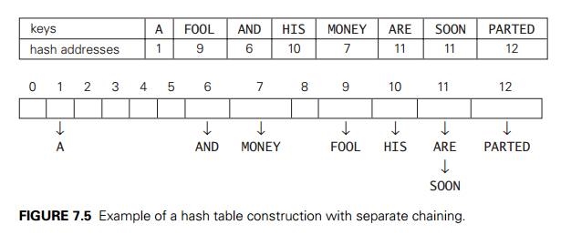
In open hashing, keys are stored in linked lists attached to cells of a hash table. Each list contains all the keys hashed to its cell. Consider, as an example, the following list of words:
A, FOOL, AND, HIS, MONEY, ARE, SOON, PARTED.
As a hash function, we will use the simple function for strings mentioned above, i.e., we will add the positions of a word’s letters in the alphabet and compute the sum’s remainder after division by 13.
We start with the empty table. The first key is the word A; its hash value is h(A) = 1 mod 13 = 1. The second key—the word FOOL—is installed in the ninth cell since (6 + 15 + 15 + 12) mod 13 = 9, and so on. The final result of this process is given in Figure 7.5; note a collision of the keys ARE and SOON because h(ARE) = (1 + 18 + 5) mod 13 = 11 and h(SOON) = (19 + 15 + 15 + 14) mod 13 = 11.
How do we search in a dictionary implemented as such a table of linked lists? We do this by simply applying to a search key the same procedure that was used for creating the table. To illustrate, if we want to search for the key KID in the hash table of Figure 7.5, we first compute the value of the same hash function for the key: h(KID) = 11. Since the list attached to cell 11 is not empty, its linked list may contain the search key. But because of possible collisions, we cannot tell whether this is the case until we traverse this linked list. After comparing the string KID first with the string ARE and then with the string SOON, we end up with an unsuccessful search.
In general, the efficiency of searching depends on the lengths of the linked lists, which, in turn, depend on the dictionary and table sizes, as well as the quality

of the hash function. If the hash function distributes n keys among m cells of the hash table about evenly, each list will be about n/m keys long. The ratio α = n/m, called the load factor of the hash table, plays a crucial role in the efficiency of hashing. In particular, the average number of pointers (chain links) inspected in successful searches, S, and unsuccessful searches, U, turns out to be

respectively, under the standard assumptions of searching for a randomly selected element and a hash function distributing keys uniformly among the table’s cells. These results are quite natural. Indeed, they are almost identical to searching sequentially in a linked list; what we have gained by hashing is a reduction in average list size by a factor of m, the size of the hash table.
Normally, we want the load factor to be not far from 1. Having it too small would imply a lot of empty lists and hence inefficient use of space; having it too large would mean longer linked lists and hence longer search times. But if we do have the load factor around 1, we have an amazingly efficient scheme that makes it possible to search for a given key for, on average, the price of one or two comparisons! True, in addition to comparisons, we need to spend time on computing the value of the hash function for a search key, but it is a constant-time operation, independent from n and m. Note that we are getting this remarkable efficiency not only as a result of the method’s ingenuity but also at the expense of extra space.
The two other dictionary operations—insertion and deletion—are almost identical to searching. Insertions are normally done at the end of a list (but see Problem 6 in this section’s exercises for a possible modification of this rule). Deletion is performed by searching for a key to be deleted and then removing it from its list. Hence, the efficiency of these operations is identical to that of searching, and they are all (1) in the average case if the number of keys n is about equal to the hash table’s size m.
Closed Hashing (Open Addressing)
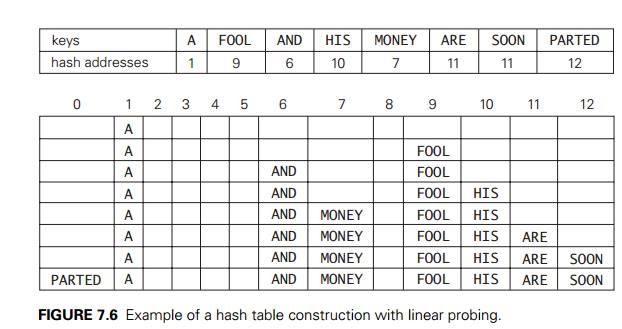
In closed hashing, all keys are stored in the hash table itself without the use of linked lists. (Of course, this implies that the table size m must be at least as large as the number of keys n.) Different strategies can be employed for collision resolution. The simplest one—called linear probing—checks the cell following the one where the collision occurs. If that cell is empty, the new key is installed there; if the next cell is already occupied, the availability of that cell’s immediate successor is checked, and so on. Note that if the end of the hash table is reached, the search is wrapped to the beginning of the table; i.e., it is treated as a circular array. This method is illustrated in Figure 7.6 with the same word list and hash function used above to illustrate separate chaining.
To search for a given key K, we start by computing h(K) where h is the hash function used in the table construction. If the cell h(K) is empty, the search is unsuccessful. If the cell is not empty, we must compare K with the cell’s occupant: if they are equal, we have found a matching key; if they are not, we compare K with a key in the next cell and continue in this manner until we encounter either a matching key (a successful search) or an empty cell (unsuccessful search). For example, if we search for the word LIT in the table of Figure 7.6, we will get h(LIT) = (12 + 9 + 20) mod 13 = 2 and, since cell 2 is empty, we can stop immediately. However, if we search for KID with h(KID) = (11 + 9 + 4) mod 13 = 11, we will have to compare KID with ARE, SOON, PARTED, and A before we can declare the search unsuccessful.
Although the search and insertion operations are straightforward for this version of hashing, deletion is not. For example, if we simply delete the key ARE from the last state of the hash table in Figure 7.6, we will be unable to find the key SOON afterward. Indeed, after computing h(SOON) = 11, the algorithm would find this location empty and report the unsuccessful search result. A simple solution
is to use “lazy deletion,” i.e., to mark previously occupied locations by a special symbol to distinguish them from locations that have not been occupied.
The mathematical analysis of linear probing is a much more difficult problem than that of separate chaining. The simplified versions of these results state that the average number of times the algorithm must access the hash table with the load factor α in successful and unsuccessful searches is, respectively,

(and the accuracy of these approximations increases with larger sizes of the hash table). These numbers are surprisingly small even for densely populated tables, i.e., for large percentage values of α:

Still, as the hash table gets closer to being full, the performance of linear probing deteriorates because of a phenomenon called clustering. A cluster in linear probing is a sequence of contiguously occupied cells (with a possible wrapping). For example, the final state of the hash table of Figure 7.6 has two clusters. Clusters are bad news in hashing because they make the dictionary operations less efficient. As clusters become larger, the probability that a new element will be attached to a cluster increases; in addition, large clusters increase the probability that two clusters will coalesce after a new key’s insertion, causing even more clustering.
Several other collision resolution strategies have been suggested to alleviate this problem. One of the most important is double hashing. Under this scheme, we use another hash function, s(K), to determine a fixed increment for the probing sequence to be used after a collision at location l = h(K):
(l + s(K)) mod m, (l + 2s(K)) mod m, . . . . (7.6)
To guarantee that every location in the table is probed by sequence (7.6), the increment s(k) and the table size m must be relatively prime, i.e., their only common divisor must be 1. (This condition is satisfied automatically if m itself is prime.) Some functions recommended in the literature are s(k) = m − 2 − k mod (m − 2) and s(k) = 8 − (k mod 8) for small tables and s(k) = k mod 97 + 1 for larger ones.
Mathematical analysis of double hashing has proved to be quite difficult. Some partial results and considerable practical experience with the method suggest that with good hashing functions—both primary and secondary—double hashing is superior to linear probing. But its performance also deteriorates when the table gets close to being full. A natural solution in such a situation is rehashing: the current table is scanned, and all its keys are relocated into a larger table.
It is worthwhile to compare the main properties of hashing with balanced search trees—its principal competitor for implementing dictionaries.
Asymptotic time efficiency with hashing, searching, insertion, and deletion can be implemented to take (1) time on the average but (n) time in the very unlikely worst case. For balanced search trees, the average time efficiencies are (log n) for both the average and worst cases.
Ordering preservation Unlike balanced search trees, hashing does not assume existence of key ordering and usually does not preserve it. This makes hashing less suitable for applications that need to iterate over the keys in or-der or require range queries such as counting the number of keys between some lower and upper bounds.
Since its discovery in the 1950s by IBM researchers, hashing has found many important applications. In particular, it has become a standard technique for storing a symbol table—a table of a computer program’s symbols generated during compilation. Hashing is quite handy for such AI applications as checking whether positions generated by a chess-playing computer program have already been considered. With some modifications, it has also proved to be useful for storing very large dictionaries on disks; this variation of hashing is called extendible hashing. Since disk access is expensive compared with probes performed in the main memory, it is preferable to make many more probes than disk accesses. Accordingly, a location computed by a hash function in extendible hashing indicates a disk ad-dress of a bucket that can hold up to b keys. When a key’s bucket is identified, all its keys are read into main memory and then searched for the key in question.
Perfect hashing is defined as a model of hashing in which any set of n elements can be stored in a hash table of equal size and can have lookups performed in constant time. It was specifically invented and discussed by Fredman, Komlos and Szemeredi (1984) and has therefore been nicknamed as "FKS Hashing".
Static Hashing defines another form of the hashing problem which permits users to accomplish lookups on a finalized dictionary set (that means all objects in the dictionary are final as well as not changing).
Since static hashing needs that the database, its objects and reference remain the same its applications are limited. Databases which contain information which experiences rare change are also eligible as it would only require a full rehash of the whole database on rare occasion. Various examples of this hashing scheme include sets of words and definitions of specific languages, sets of significant data for an organization's personnel, etc.
In the static case, we are provided a set with a total of p entries, each one associated with a unique key, ahead of time. Fredman, Komlós and Szemerédi select a first-level hash table with size s = 2(p-1) buckets. To construct, p entries are separated into q buckets by the top-level hashing function, where q = 2(p-1). Then for each bucket with r entries, a second-level table is allocated with r2 slots, and its hash function is chosen at random from a universal hash function set so that it becomes collision-free and stored alongside the hash table. If the hash function randomly chosen creates a table with collisions, a new hash function is randomly chosen until a collision-free table can be guaranteed. At last, with the collision-free hash, the r entries are hashed into the second-level table.
1.3.8 Load Factor and Rehashing
For insertion of a key(K) – value(V) pair into a hash map, 2 steps are required:
For example, if the key is a string “abcd”, then it’s hash function may depend on the length of the string. But for very large values of n, the number of entries into the map, length of the keys is almost negligible in comparison to n so hash computation can be considered to take place in constant time, i.e, O(1).
As the name suggests, rehashing means hashing again. Basically, when the load factor increases to more than its pre-defined value (default value of load factor is 0.75), the complexity increases. So to overcome this, the size of the array is increased (doubled) and all the values are hashed again and stored in the new double sized array to maintain a low load factor and low complexity.
Why rehashing?Rehashing is done because whenever key value pairs are inserted into the map, the load factor increases, which implies that the time complexity also increases as explained above. This might not give the required time complexity of O(1).
Hence, rehash must be done, increasing the size of the bucketArray so as to reduce the load factor and the time complexity.
How Rehashing is done?Rehashing can be done as follows:
Program to implement Rehashing:
// Java program to implement Rehashing
import java.util.ArrayList;
class Map<K, V> {
class MapNode<K, V> {
K key; V value; MapNode<K, V> next;
public MapNode(K key, V value) { this.key = key; this.value = value; next = null; } }
// The bucket array where // the nodes containing K-V pairs are stored ArrayList<MapNode<K, V> > buckets;
// No. of pairs stored - n int size;
// Size of the bucketArray - b int numBuckets;
// Default loadFactor final double DEFAULT_LOAD_FACTOR = 0.75;
public Map() { numBuckets = 5;
buckets = new ArrayList<>(numBuckets);
for (int i = 0; i < numBuckets; i++) { // Initialising to null buckets.add(null); } System.out.println("HashMap created"); System.out.println("Number of pairs in the Map: " + size); System.out.println("Size of Map: " + numBuckets); System.out.println("Default Load Factor: " + DEFAULT_LOAD_FACTOR + "\n"); }
private int getBucketInd(K key) {
// Using the inbuilt function from the object class int hashCode = key.hashCode();
// array index = hashCode%numBuckets return (hashCode % numBuckets); }
public void insert(K key, V value) { // Getting the index at which, it needs to be inserted int bucketInd = getBucketInd(key);
// The first node at that index MapNode<K, V> head = buckets.get(bucketInd);
// First, loop through all the nodes present at that index // to check if the key already exists while (head != null) {
// If already present the value is updated if (head.key.equals(key)) { head.value = value; return; } head = head.next; }
// new node with the K and V MapNode<K, V> newElementNode = new MapNode<K, V>(key, value);
// The head node at the index head = buckets.get(bucketInd);
// the new node is inserted // by making it the head // and it's next is the previous head newElementNode.next = head;
buckets.set(bucketInd, newElementNode);
System.out.println("Pair(" + key + ", " + value + ") inserted successfully.\n");
// Incrementing size // as new K-V pair is added to the map size++;
// Load factor calculated double loadFactor = (1.0 * size) / numBuckets;
System.out.println("Current Load factor = " + loadFactor);
// If the load factor is > 0.75, rehashing is done if (loadFactor > DEFAULT_LOAD_FACTOR) { System.out.println(loadFactor + " is greater than " + DEFAULT_LOAD_FACTOR); System.out.println("Therefore Rehashing will be done.\n");
// Rehash rehash();
System.out.println("New Size of Map: " + numBuckets + "\n"); }
System.out.println("Number of pairs in the Map: " + size); System.out.println("Size of Map: " + numBuckets + "\n"); }
private void rehash() {
System.out.println("\n***Rehashing Started***\n");
// The present bucket list is made temp ArrayList<MapNode<K, V> > temp = buckets;
// New bucketList of double the old size is created buckets = new ArrayList<MapNode<K, V> >(2 * numBuckets);
for (int i = 0; i < 2 * numBuckets; i++) { // Initialised to null buckets.add(null); } // Now size is made zero // and we loop through all the nodes in the original bucket list(temp) // and insert it into the new list size = 0; numBuckets *= 2;
for (int i = 0; i < temp.size(); i++) {
// head of the chain at that index MapNode<K, V> head = temp.get(i);
while (head != null) { K key = head.key; V val = head.value;
// calling the insert function for each node in temp // as the new list is now the bucketArray insert(key, val); head = head.next; } }
System.out.println("\n***Rehashing Ended***\n"); }
public void printMap() {
// The present bucket list is made temp ArrayList<MapNode<K, V> > temp = buckets;
System.out.println("Current HashMap:"); // loop through all the nodes and print them for (int i = 0; i < temp.size(); i++) {
// head of the chain at that index MapNode<K, V> head = temp.get(i);
while (head != null) { System.out.println("key = " + head.key + ", val = " + head.value);
head = head.next; } } System.out.println(); } }
public class GFG {
public static void main(String[] args) {
// Creating the Map Map<Integer, String> map = new Map<Integer, String>();
// Inserting elements map.insert(1, "Geeks"); map.printMap();
map.insert(2, "forGeeks"); map.printMap();
map.insert(3, "A"); map.printMap();
map.insert(4, "Computer"); map.printMap();
map.insert(5, "Portal"); map.printMap(); } } |
Output:
HashMap created
Number of pairs in the Map: 0
Size of Map: 5
Default Load Factor: 0.75
Pair(1, Geeks) inserted successfully.
Current Load factor = 0.2
Number of pairs in the Map: 1
Size of Map: 5
Current HashMap:
key = 1, val = Geeks
Pair(2, forGeeks) inserted successfully.
Current Load factor = 0.4
Number of pairs in the Map: 2
Size of Map: 5
Current HashMap:
key = 1, val = Geeks
key = 2, val = forGeeks
Pair(3, A) inserted successfully.
Current Load factor = 0.6
Number of pairs in the Map: 3
Size of Map: 5
Current HashMap:
key = 1, val = Geeks
key = 2, val = forGeeks
key = 3, val = A
Pair(4, Computer) inserted successfully.
Current Load factor = 0.8
0.8 is greater than 0.75
Therefore Rehashing will be done.
***Rehashing Started***
Pair(1, Geeks) inserted successfully.
Current Load factor = 0.1
Number of pairs in the Map: 1
Size of Map: 10
Pair(2, forGeeks) inserted successfully.
Current Load factor = 0.2
Number of pairs in the Map: 2
Size of Map: 10
Pair(3, A) inserted successfully.
Current Load factor = 0.3
Number of pairs in the Map: 3
Size of Map: 10
Pair(4, Computer) inserted successfully.
Current Load factor = 0.4
Number of pairs in the Map: 4
Size of Map: 10
***Rehashing Ended***
New Size of Map: 10
Number of pairs in the Map: 4
Size of Map: 10
Current HashMap:
key = 1, val = Geeks
key = 2, val = forGeeks
key = 3, val = A
key = 4, val = Computer
Pair(5, Portal) inserted successfully.
Current Load factor = 0.5
Number of pairs in the Map: 5
Size of Map: 10
Current HashMap:
key = 1, val = Geeks
key = 2, val = forGeeks
key = 3, val = A
key = 4, val = Computer
key = 5, val = Portal
The Sum of Functions Problem
Given a set A and a function f, whose domain contains A and which can be calculated in time O(1), find all non-trivial quadruples (x, y, z, w) of elements x, y, z, w ∈ A such that f(x) + f(y) = f(z) + f(w).
For a trivial solution, we may simply test each quadruple of distinct elements of the set A. We can do this in Θ(n 4) time, where n = |A|.
A more efficient solution can be achieved by sorting. Pick all pairs (x, y) ⊂ A, put them on a list L, and sort them by d x,y = f(x) + f(y). Now, all pairs of elements whose images under f sum up to a same value d will constitute a contiguous sublist of L. Therefore, they can be easily combined to produce the intended quadruples in constant time per quadruple. Owing to sorting, the overall time complexity of this approach is O(n 2 log n + q), in the worst case, where q is the number of quadruples in the output.1
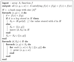
Now we look into a hashing-based approach. We start with an empty hash map H. We consider each unordered pair (x, y) of distinct elements of A, obtaining d = f(x) + f(y), one pair at a time. If d is not a key stored in H, we insert the (key, value) pair (d, S d) in H, where S d is a collection (which can be implemented as a linked list, a hash set or whatever other structure) containing only the pair (x, y) initially. On the other hand, if d is already stored in H, then we simply add (x, y) to the non-empty collection S d which d already maps to in H. After all pairs of distinct elements have been considered, our hash map will contain non-empty collections S d whose elements are pairs (x, y) satisfying f(x) + f(y) = d. For each non-unitary collection Sd, we combine distinct pairs (x, y), (z, w) ∈ S d , two at a time, to produce our desired quadruples (x, y, z, w).
The pseudocode of the proposed hash-based solution.
Algorithm 1 Sum Functions (A, f).
As for the time complexity of the algorithm, each key d can be located or inserted in H in O(1) average time, and each of the Θ(n 2) pairs (x, y) of elements of A can be inserted in some list S d in O(1) time (assuming, for instance, a linked list implementation for S d ). Thus, the whole step of populating H can be performed in Θ(n 2) time on average. Now, each of the q quadruples that satisfy the equality can be obtained, by combining pairs in a same list, in O(1) time. Thus, the whole algorithm runs in Θ(n 2 + q) expected time.
If we tried to achieve the same performance by using an array and direct addressing, such array would have to be twice as large as the maximum element in the image of f. The use of hashing avoids that issue seamlessly.
In the standard game of bingo, each of the contestants receives a card with some integers. The integers in each card constitute a subset of a rather small range A = [1, a]. Then, subsequent numbers are drawn at random from A, without replacement, until all numbers in the card of a contestant have been drawn. That contestant wins the prize.
In our variation of the game, the contestants receive an empty card. Subsequent numbers are drawn at random from some unknown, huge range B = [1, b], with replacement, forming a sequence S. The contestant who wins the game is the one who first spots a set W = {x, y, z} of three distinct numbers such that all 3! = 6 permutations of its elements appear among the subsequences of three consecutive elements of S. As an example, the sequence
S = (2, 19, 4, 1, 100, 1, 4, 19, 1, 4, 1, 19, 100, 192, 100, 4, 19, 2, 1, 19, 4)
is a minimal winning sequence. There is a set, namely W = {1, 4, 19}, such that every permutation of W appears as three consecutive elements of S. Even though the set B is huge, the distribution of the drawing probability along B is not uniform, and the game finishes in reasonable time almost surely.
We want to write a program to play the permutation bingo. Moreover, we want our program to win the game when it plays against other programs. In other words, we need an efficient algorithm to check, after each number is added to S, whether S happens to be a winning sequence.
One possible approach would be as follows. Keep S in memory all the time. After the n-th number is added, for all n ≥ 8 (a trivial lower bound for the size of a winning sequence), traverse S = (s 1, s 2, ..., s n ) entirely for each set R i = {s i , s i+1 , s i+2 } of three consecutive distinct elements (with 1≤ i ≤ n - 2), checking whether all permutations of R i appear as consecutive elements of S. Checking a sequence of size n this way demands Θ(n 2) time in the worst case.
We can do better by performing a single traversal of S, during which we add each subsequence of three consecutive distinct elements of S into a bin. To make sure that two permutations go to the same bin if and only if they have the same elements (in different orders), we may label each bin using the ascending sequence of its elements. Now, for each subsequence of three distinct elements in S, we compute the label of its bin, find the bin, and place the subsequence therein, making sure we do not add the same subsequence twice in a bin. Whenever a bin has size six, we have a winner. We can implement each bin labeled (x, y, z), with x < y < z, using an array of integers, or a linked list, or a hash set, or even a bit array if we care to compute the position of any given permutation in a total order of the permutations of those elements. As a matter of fact, the way we implement each bin is not important, since its size will never exceed six. Moreover, rather than building the bins from scratch by traversing the whole S each time a new element s n is added, we can keep the bins in memory and proceed to place only each freshly formed subsequence (s n-2 , s n-1 , s n ) into the appropriate bin - an approach which also allows us to keep but the two last elements of S in memory.
We still have a big problem, though. Given a label, how to find the bin among the (possibly huge number of) existing bins? If we maintain, say, an array of bins, then we will have to traverse that entire array until we find the desired bin. It is not even possible to attempt direct addressing here, for the range B of the numbers that can be drawn is not only unknown but also possibly huge - let alone the number of subsets of three such numbers! Even if we did know B, there would probably not be enough available memory for such an array. We know, however, that the game always ends in reasonable time, owing to an appropriate probability distribution along B enforced by the game dealer. Thus, the actual number of bins that will ever be used is small, and available memory to store only that number of bins shall not be an issue. We can therefore keep the bins in a linked list, or even in an array without direct addressing. When the sequence has size n, such list (or array) of bins will have size O(n), and the time it takes to traverse it all and find the desired bin will also be O(n).
The use of hashing can improve the performance even further. We use a hash map where the keys are the bin labels and the values are the bins themselves (each one a list, or bit array etc.), so every time a new element is added, we can find the appropriate bin and update its contents in expected constant time. Since we do not know the number of bins that will be stored in our hash map throughout the game, and we want to keep the load factor of the hash map below a certain constant, we implement the hash map over an initially small dynamic array and adopt a geometric expansion policy to resize it whenever necessary. By doing this, the amortized cost of inserting each new bin is also constant, and the algorithm processes each drawn number in overall O(1) expected time.
The Ferry Loading Problem (FLP) is not unknown to those used to international programming competitions. It appears in the chapter devoted to dynamic programming, the technique employed in the generally accepted, pseudo-polynomial solution. By using a clever backtracking approach aided by hashing, we obtain a simpler algorithm which is just as efficient, in the worst case. As a matter of fact, our algorithm may demand significantly less time and space, in practice, than the usual dynamic programming approach.
There is a ferry to transport cars across a river. The ferry comprises two lanes of cars throughout its length. Before boarding on the ferry, the cars wait on a single queue in their order of arrival. When boarding, each car goes either to the left or to the right lane at the discretion of the ferry operator. Whenever the next car in the queue cannot be boarded on either lane, the ferry departs, and all cars still in the queue should wait for the next ferry. Given the length L ∈ ℤ of the ferry and the lengths ℓ i ∈ ℤ of all cars i > 0 in the queue, the problem asks for the maximum number of cars that can be loaded onto the ferry.
A brute force approach could be as follows. Starting from k = 1, attempt all 2k distributions of the first k cars in the queue. If it is possible to load k cars on the ferry, proceed with the next value of k. Stop when there is no feasible distribution of cars for some k. Clearly, if the number n of cars loaded in the optimal solution is not ridiculously small, such an exponential-time algorithm is doomed to run for ages.
A dynamic programming strategy can be devised to solve the FLP in Θ(nL) time and space. This is not surprising, given the similarity of this problem with the Knapsack Problem, the Partition Problem, and the Bin Packing Problem. Such complexity, as usual, corresponds to the size of the dynamic programming table that must be filled with answers to subproblems, each one computed in constant time.
Apart from the dynamic programming approach, one could come up with a simple backtracking strategy as follows. Identify each feasible configuration of k cars by a tuple (x 1, ..., x k), where x i ∈ {left, right} indicates the lane occupied by the ith car, for i = 1, ..., k. Each configuration (x 1, ..., x k) leads to configurations (x 1, ..., x k, left) and (x 1, ..., x k, right), respectively, if there is room for the (k + 1)th car on the corresponding lane. Starting from the configuration (left) - the first car boards on the left lane, without loss of generality -, inspect all feasible configurations in backtracking fashion and report the size of the largest configuration that is found. It works fine. Unfortunately, such approach demands exponential time in the worst case.
However, we can perfectly well identify each configuration by a pair (k, s), where k is the number of cars on the ferry and s is the total length of the left lane that is occupied by cars. Each configuration (k, s) leads to at most two other configurations in the implicit backtracking graph:

If neither placement of the (k + 1)th car is possible, backtrack. Notice that a same configuration (k + 1, s') may be reached by two distinct configurations (k, s 1) and (k, s 2). It happens precisely if |s 1 - s 2| = ℓ k+1 . However, we do not want to visit a same configuration twice, and therefore we must keep track of the visited configurations.
The algorithm searches the whole backtracking graph, starting by the root node (0, 0) - there are zero cars on the ferry, initially, occupying zero space on the left lane. The reported solution will be the largest k that is found among the visited configurations (k, s).
As for the time complexity, the whole search runs in time proportional to the number of nodes (configurations) in the backtracking graph. Since 0 ≤ k ≤ n, 0 ≤ s ≤ L, and both k and s are integers, such number is O(nL), bounding the worst-case time complexity of our algorithm if we make sure we can check whether a configuration has already been visited in O(1) time. If we use a 2-dimensional matrix to store the configurations, the problem is solved. However, by doing so, we demand Θ(nL) space, even though our matrix will most likely be absolutely sparse.
We can resort to hashing to solve that. By using a hash set to store the visited configurations, we can still perform each configuration lookup in (expected) constant time, and the required space will be proportional to the number O(nL) of configurations that are actually visited during the search. In practice, the O(nL) time and space required by our algorithm can be remarkably smaller than the Θ(nL) time and space of the dynamic programming solution, especially if there are many cars with the same size.
Key takeaway
Following are the basic primary operations of a hash table.
Hash Function is used to index the original value or key and then used later each time the data associated with the value or key is to be retrieved. Thus, hashing is always a one-way operation. There is no need to "reverse engineer" the hash function by analyzing the hashed values.
Characteristics of Good Hash Function:
Some Popular Hash Function is:
Choose a number m smaller than the number of n of keys in k (The number m is usually chosen to be a prime number or a number without small divisors, since this frequently a minimum number of collisions).
The hash function is:

For Example: if the hash table has size m = 12 and the key is k = 100, then h (k) = 4. Since it requires only a single division operation, hashing by division is quite fast.
The multiplication method for creating hash functions operates in two steps. First, we multiply the key k by a constant A in the range 0 < A < 1 and extract the fractional part of kA. Then, we increase this value by m and take the floor of the result.
The hash function is:

Where "k A mod 1" means the fractional part of k A, that is, k A -⌊k A⌋.
The key k is squared. Then function H is defined by
Where L is obtained by deleting digits from both ends of k2. We emphasize that the same position of k2 must be used for all of the keys.
The key k is partitioned into a number of parts k1, k2.... kn where each part except possibly the last, has the same number of digits as the required address.
Then the parts are added together, ignoring the last carry.
H (k) = k1+ k2+.....+kn
Example: Company has 68 employees, and each is assigned a unique four- digit employee number. Suppose L consist of 2- digit addresses: 00, 01, and 02....99. We apply the above hash functions to each of the following employee numbers:
(a) Division Method: Choose a Prime number m close to 99, such as m =97, Then
That is dividing 3205 by 17 gives a remainder of 4, dividing 7148 by 97 gives a remainder of 67, dividing 2345 by 97 gives a remainder of 17.
(b) Mid-Square Method:
k = 3205 7148 2345
k2= 10272025 51093904 5499025
h (k) = 72 93 99
Observe that fourth & fifth digits, counting from right are chosen for hash address.
(c) Folding Method: Divide the key k into 2 parts and adding yields the following hash address:
Key takeaway
Hash Function is used to index the original value or key and then used later each time the data associated with the value or key is to be retrieved. Thus, hashing is always a one-way operation. There is no need to "reverse engineer" the hash function by analyzing the hashed values.
Characteristics of Good Hash Function:
Collision Resolution Techniques
Collision resolution techniques
There are two types of collision resolution techniques.
In this technique, a linked list is created from the slot in which collision has occurred, after which the new key is inserted into the linked list. This linked list of slots looks like a chain, so it is called separate chaining. It is used more when we do not know how many keys to insert or delete.
Time complexityAdvantages of separate chaining
Disadvantages of separate chaining
Open addressing is collision-resolution method that is used to control the collision in the hashing table. There is no key stored outside of the hash table. Therefore, the size of the hash table is always greater than or equal to the number of keys. It is also called closed hashing.
The following techniques are used in open addressing:
In this, when the collision occurs, we perform a linear probe for the next slot, and this probing is performed until an empty slot is found. In linear probing, the worst time to search for an element is O(table size). The linear probing gives the best performance of the cache but its problem is clustering. The main advantage of this technique is that it can be easily calculated.
Disadvantages of linear probing
In this, when the collision occurs, we probe for i2th slot in ith iteration, and this probing is performed until an empty slot is found. The cache performance in quadratic probing is lower than the linear probing. Quadratic probing also reduces the problem of clustering.
In this, you use another hash function, and probe for (i * hash 2(x)) in the ith iteration. It takes longer to determine two hash functions. The double probing gives the very poor the cache performance, but there has no clustering problem in it.
Key takeaway
An overflow occurs at the time of the home bucket for a new pair (key, element) is full.
We may tackle overflows by
Search the hash table in some systematic manner for a bucket that is not full.
Eliminate overflows by allowing each bucket to keep a list of all pairs for which it is the home bucket.
Open addressing is performed to ensure that all elements are stored directly into the hash table, thus it attempts to resolve collisions implementing various methods.
Linear Probing is performed to resolve collisions by placing the data into the next open slot in the table.
Linear probing searches buckets (H(x)+i2)%b; H(x) indicates Hash function of x
Quadratic probing implements a quadratic function of i as the increment
Examine buckets H(x), (H(x)+i2)%b, (H(x)-i2)%b, for 1<=i<=(b-1)/2
b is indicated as a prime number of the form 4j+3, j is an integer
Random Probing performs incorporating with random numbers.
H(x):= (H’(x) + S[i]) % b
S[i] is a table along with size b-1
S[i] is indicated as a random permutation of integers [1, b-1].
Hashing
In this section, we consider a very efficient way to implement dictionaries. Recall that a dictionary is an abstract data type, namely, a set with the operations of searching (lookup), insertion, and deletion defined on its elements. The elements of this set can be of an arbitrary nature: numbers, characters of some alphabet, character strings, and so on. In practice, the most important case is that of records (student records in a school, citizen records in a governmental office, book records in a library).
Typically, records comprise several fields, each responsible for keeping a particular type of information about an entity the record represents. For example, a student record may contain fields for the student’s ID, name, date of birth, sex, home address, major, and so on. Among record fields there is usually at least one called a key that is used for identifying entities represented by the records (e.g., the student’s ID). In the discussion below, we assume that we have to implement a dictionary of n records with keys K1, K2, . . . , Kn.
Hashing is based on the idea of distributing keys among a one-dimensional array H [0..m − 1] called a hash table. The distribution is done by computing, for each of the keys, the value of some predefined function h called the hash function. This function assigns an integer between 0 and m − 1, called the hash address, to a key.
For example, if keys are nonnegative integers, a hash function can be of the form h(K) = K mod m; obviously, the remainder of division by m is always between 0 and m − 1. If keys are letters of some alphabet, we can first assign a letter its position in the alphabet, denoted here ord(K), and then apply the same kind of a function used for integers. Finally, if K is a character string

where C is a constant larger than every ord(ci).
In general, a hash function needs to satisfy somewhat conflicting require-ments:
A hash table’s size should not be excessively large compared to the number of keys, but it should be sufficient to not jeopardize the implementation’s time efficiency (see below).
A hash function needs to distribute keys among the cells of the hash table as evenly as possible. (This requirement makes it desirable, for most applications, to have a hash function dependent on all bits of a key, not just some of them.)
A hash function has to be easy to compute.

Obviously, if we choose a hash table’s size m to be smaller than the number of keys n, we will get collisions—a phenomenon of two (or more) keys being hashed into the same cell of the hash table (Figure 7.4). But collisions should be expected even if m is considerably larger than n (see Problem 5 in this section’s exercises). In fact, in the worst case, all the keys could be hashed to the same cell of the hash table. Fortunately, with an appropriately chosen hash table size and a good hash function, this situation happens very rarely. Still, every hashing scheme must have a collision resolution mechanism. This mechanism is different in the two principal versions of hashing: open hashing (also called separate chaining) and closed hashing (also called open addressing).
Open Hashing (Separate Chaining)
In open hashing, keys are stored in linked lists attached to cells of a hash table. Each list contains all the keys hashed to its cell. Consider, as an example, the following list of words:
A, FOOL, AND, HIS, MONEY, ARE, SOON, PARTED.
As a hash function, we will use the simple function for strings mentioned above, i.e., we will add the positions of a word’s letters in the alphabet and compute the sum’s remainder after division by 13.
We start with the empty table. The first key is the word A; its hash value is h(A) = 1 mod 13 = 1. The second key—the word FOOL—is installed in the ninth cell since (6 + 15 + 15 + 12) mod 13 = 9, and so on. The final result of this process is given in Figure 7.5; note a collision of the keys ARE and SOON because h(ARE) = (1 + 18 + 5) mod 13 = 11 and h(SOON) = (19 + 15 + 15 + 14) mod 13 = 11.
How do we search in a dictionary implemented as such a table of linked lists? We do this by simply applying to a search key the same procedure that was used for creating the table. To illustrate, if we want to search for the key KID in the hash table of Figure 7.5, we first compute the value of the same hash function for the key: h(KID) = 11. Since the list attached to cell 11 is not empty, its linked list may contain the search key. But because of possible collisions, we cannot tell whether this is the case until we traverse this linked list. After comparing the string KID first with the string ARE and then with the string SOON, we end up with an unsuccessful search.
In general, the efficiency of searching depends on the lengths of the linked lists, which, in turn, depend on the dictionary and table sizes, as well as the quality
of the hash function. If the hash function distributes n keys among m cells of the hash table about evenly, each list will be about n/m keys long. The ratio α = n/m, called the load factor of the hash table, plays a crucial role in the efficiency of hashing. In particular, the average number of pointers (chain links) inspected in successful searches, S, and unsuccessful searches, U, turns out to be

respectively, under the standard assumptions of searching for a randomly selected element and a hash function distributing keys uniformly among the table’s cells. These results are quite natural. Indeed, they are almost identical to searching sequentially in a linked list; what we have gained by hashing is a reduction in average list size by a factor of m, the size of the hash table.
Normally, we want the load factor to be not far from 1. Having it too small would imply a lot of empty lists and hence inefficient use of space; having it too large would mean longer linked lists and hence longer search times. But if we do have the load factor around 1, we have an amazingly efficient scheme that makes it possible to search for a given key for, on average, the price of one or two comparisons! True, in addition to comparisons, we need to spend time on computing the value of the hash function for a search key, but it is a constant-time operation, independent from n and m. Note that we are getting this remarkable efficiency not only as a result of the method’s ingenuity but also at the expense of extra space.
The two other dictionary operations—insertion and deletion—are almost identical to searching. Insertions are normally done at the end of a list (but see Problem 6 in this section’s exercises for a possible modification of this rule). Deletion is performed by searching for a key to be deleted and then removing it from its list. Hence, the efficiency of these operations is identical to that of searching, and they are all (1) in the average case if the number of keys n is about equal to the hash table’s size m.
Closed Hashing (Open Addressing)
In closed hashing, all keys are stored in the hash table itself without the use of linked lists. (Of course, this implies that the table size m must be at least as large as the number of keys n.) Different strategies can be employed for collision resolution. The simplest one—called linear probing—checks the cell following the one where the collision occurs. If that cell is empty, the new key is installed there; if the next cell is already occupied, the availability of that cell’s immediate successor is checked, and so on. Note that if the end of the hash table is reached, the search is wrapped to the beginning of the table; i.e., it is treated as a circular array. This method is illustrated in Figure 7.6 with the same word list and hash function used above to illustrate separate chaining.
To search for a given key K, we start by computing h(K) where h is the hash function used in the table construction. If the cell h(K) is empty, the search is unsuccessful. If the cell is not empty, we must compare K with the cell’s occupant: if they are equal, we have found a matching key; if they are not, we compare K with a key in the next cell and continue in this manner until we encounter either a matching key (a successful search) or an empty cell (unsuccessful search). For example, if we search for the word LIT in the table of Figure 7.6, we will get h(LIT) = (12 + 9 + 20) mod 13 = 2 and, since cell 2 is empty, we can stop immediately. However, if we search for KID with h(KID) = (11 + 9 + 4) mod 13 = 11, we will have to compare KID with ARE, SOON, PARTED, and A before we can declare the search unsuccessful.
Although the search and insertion operations are straightforward for this version of hashing, deletion is not. For example, if we simply delete the key ARE from the last state of the hash table in Figure 7.6, we will be unable to find the key SOON afterward. Indeed, after computing h(SOON) = 11, the algorithm would find this location empty and report the unsuccessful search result. A simple solution

is to use “lazy deletion,” i.e., to mark previously occupied locations by a special symbol to distinguish them from locations that have not been occupied.
The mathematical analysis of linear probing is a much more difficult problem than that of separate chaining. The simplified versions of these results state that the average number of times the algorithm must access the hash table with the load factor α in successful and unsuccessful searches is, respectively,

(and the accuracy of these approximations increases with larger sizes of the hash table). These numbers are surprisingly small even for densely populated tables, i.e., for large percentage values of α:
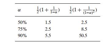
Still, as the hash table gets closer to being full, the performance of linear probing deteriorates because of a phenomenon called clustering. A cluster in linear probing is a sequence of contiguously occupied cells (with a possible wrapping). For example, the final state of the hash table of Figure 7.6 has two clusters. Clusters are bad news in hashing because they make the dictionary operations less efficient. As clusters become larger, the probability that a new element will be attached to a cluster increases; in addition, large clusters increase the probability that two clusters will coalesce after a new key’s insertion, causing even more clustering.
Several other collision resolution strategies have been suggested to alleviate this problem. One of the most important is double hashing. Under this scheme, we use another hash function, s(K), to determine a fixed increment for the probing sequence to be used after a collision at location l = h(K):
(l + s(K)) mod m, (l + 2s(K)) mod m, . . . . (7.6)
To guarantee that every location in the table is probed by sequence (7.6), the increment s(k) and the table size m must be relatively prime, i.e., their only common divisor must be 1. (This condition is satisfied automatically if m itself is prime.) Some functions recommended in the literature are s(k) = m − 2 − k mod (m − 2) and s(k) = 8 − (k mod 8) for small tables and s(k) = k mod 97 + 1 for larger ones.
Mathematical analysis of double hashing has proved to be quite difficult. Some partial results and considerable practical experience with the method suggest that with good hashing functions—both primary and secondary—double hashing is superior to linear probing. But its performance also deteriorates when the table gets close to being full. A natural solution in such a situation is rehashing: the current table is scanned, and all its keys are relocated into a larger table.
It is worthwhile to compare the main properties of hashing with balanced search trees—its principal competitor for implementing dictionaries.
Asymptotic time efficiency with hashing, searching, insertion, and deletion can be implemented to take (1) time on the average but (n) time in the very unlikely worst case. For balanced search trees, the average time efficiencies are (log n) for both the average and worst cases.
Ordering preservation Unlike balanced search trees, hashing does not assume existence of key ordering and usually does not preserve it. This makes hashing less suitable for applications that need to iterate over the keys in or-der or require range queries such as counting the number of keys between some lower and upper bounds.
Since its discovery in the 1950s by IBM researchers, hashing has found many important applications. In particular, it has become a standard technique for storing a symbol table—a table of a computer program’s symbols generated during compilation. Hashing is quite handy for such AI applications as checking whether positions generated by a chess-playing computer program have already been considered. With some modifications, it has also proved to be useful for storing very large dictionaries on disks; this variation of hashing is called extendible hashing. Since disk access is expensive compared with probes performed in the main memory, it is preferable to make many more probes than disk accesses. Accordingly, a location computed by a hash function in extendible hashing indicates a disk ad-dress of a bucket that can hold up to b keys.
Extendible Hashing is a dynamic hashing method wherein directories, and buckets are used to hash data. It is an aggressively flexible method in which the hash function also experiences dynamic changes.
Main features of Extendible Hashing: The main features in this hashing technique are:
Basic Structure of Extendible Hashing:
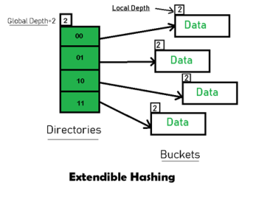
Frequently used terms in Extendible Hashing:
Basic Working of Extendible Hashing:
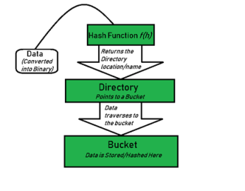
Eg. The binary obtained is: 110001 and the global-depth is 3. So, the hash function will return 3 LSBs of 110001 viz. 001.
First, Check if the local depth is less than or equal to the global depth. Then choose one of the cases below.
Directory expansion will double the number of directories present in the hash structure.
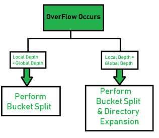
Example based on Extendible Hashing: Now, let us consider a prominent example of hashing the following elements: 16,4,6,22,24,10,31,7,9,20,26.
Bucket Size: 3 (Assume)
Hash Function: Suppose the global depth is X. Then the Hash Function returns X LSBs.
16- 10000
4- 00100
6- 00110
22- 10110
24- 11000
10- 01010
31- 11111
7- 00111
9- 01001
20- 10100
26- 01101
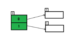
The binary format of 16 is 10000 and global-depth is 1. The hash function returns 1 LSB of 10000 which is 0. Hence, 16 is mapped to the directory with id=0.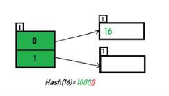
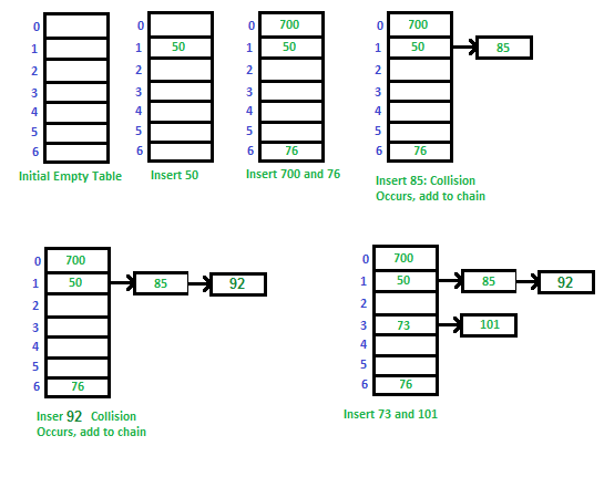
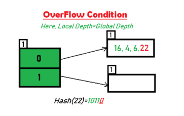
[16(10000),4(100),6(110),22(10110)]
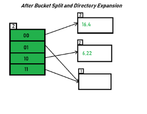
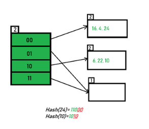
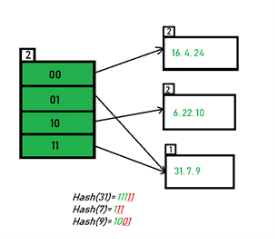
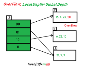
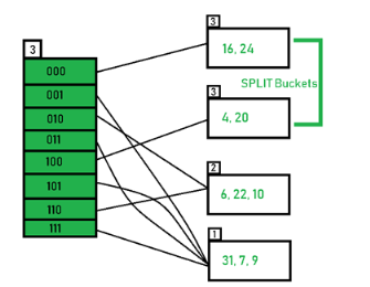
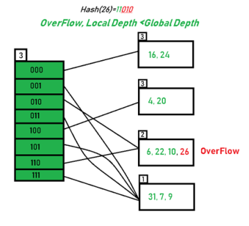
Finally, the output of hashing the given list of numbers is obtained.
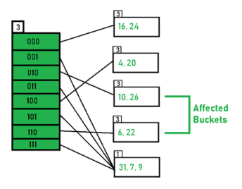
Key Observations:
is equal to the global depth, only then the directories are doubled and the global depth is incremented by 1.
4. The size of a bucket cannot be changed after the data insertion process begins.
Advantages:
Limitations of Extendible Hashing:
Key takeaway
An overflow occurs at the time of the home bucket for a new pair (key, element) is full.
We may tackle overflows by
Search the hash table in some systematic manner for a bucket that is not full.
A skip list is a probabilistic data structure. The skip list is used to store a sorted list of elements or data with a linked list. It allows the process of the elements or data to view efficiently. In one single step, it skips several elements of the entire list, which is why it is known as a skip list.
The skip list is an extended version of the linked list. It allows the user to search, remove, and insert the element very quickly. It consists of a base list that includes a set of elements which maintains the link hierarchy of the subsequent elements.
It is built in two layers: The lowest layer and Top layer.
The lowest layer of the skip list is a common sorted linked list, and the top layers of the skip list are like an "express line" where the elements are skipped.
Complexity table of the Skip list
S. No | Complexity | Average case | Worst case |
1. | Access complexity | O(logn) | O(n) |
2. | Search complexity | O(logn) | O(n) |
3. | Delete complexity | O(logn) | O(n) |
4. | Insert complexity | O(logn) | O(n) |
5. | Space complexity | - | O(nlogn) |
Let's take an example to understand the working of the skip list. In this example, we have 14 nodes, such that these nodes are divided into two layers, as shown in the diagram.
The lower layer is a common line that links all nodes, and the top layer is an express line that links only the main nodes, as you can see in the diagram.
Suppose you want to find 47 in this example. You will start the search from the first node of the express line and continue running on the express line until you find a node that is equal a 47 or more than 47.
You can see in the example that 47 does not exist in the express line, so you search for a node of less than 47, which is 40. Now, you go to the normal line with the help of 40, and search the 47, as shown in the diagram.

There are the following types of operations in the skip list.
Algorithm of the insertion operation
Algorithm of deletion operation
Algorithm of searching operation
Example 1: Create a skip list, we want to insert these following keys in the empty skip list.
Ans:
Step 1: Insert 6 with level 1
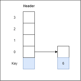
Step 2: Insert 29 with level 1
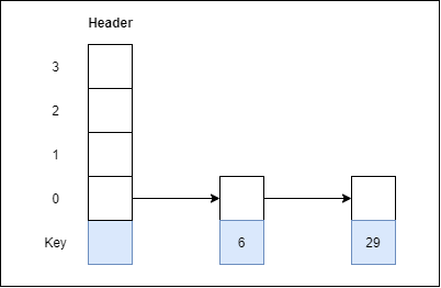
Step 3: Insert 22 with level 4
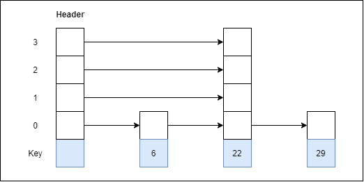
Step 4: Insert 9 with level 3
Step 5: Insert 17 with level 1
Step 6: Insert 4 with level 2

Example 2: Consider this example where we want to search for key 17.
Ans:
Disadvantages of the Skip list
Key takeaway
A skip list is a probabilistic data structure. The skip list is used to store a sorted list of elements or data with a linked list. It allows the process of the elements or data to view efficiently. In one single step, it skips several elements of the entire list, which is why it is known as a skip list.
The skip list is an extended version of the linked list. It allows the user to search, remove, and insert the element very quickly. It consists of a base list that includes a set of elements which maintains the link hierarchy of the subsequent elements.
References:
1. Horowitz, Sahani, Dinesh Mehata, ―Fundamentals of Data Structures in C++‖, Galgotia Publisher, ISBN: 8175152788, 9788175152786.
2. M Folk, B Zoellick, G. Riccardi, ―File Structures‖, Pearson Education, ISBN:81-7758-37-5
3. Peter Brass, ―Advanced Data Structures‖, Cambridge University Press, ISBN: 978-1-107- 43982-5
4. A. Aho, J. Hopcroft, J. Ulman, ―Data Structures and Algorithms‖, Pearson Education, 1998, ISBN-0-201-43578-0.
5. Michael J Folk, ―File Structures an Object-Oriented Approach with C++‖, Pearson Education, ISBN: 81-7758-373-5.
6. Sartaj Sahani, ―Data Structures, Algorithms and Applications in C++‖, Second Edition, University Press, ISBN:81-7371522 X.
7. G A V Pai, ―Data Structures and Algorithms‖, The McGraw-Hill Companies, ISBN - 9780070667266.
8. Goodrich, Tamassia, Goldwasser, ―Data Structures and Algorithms in Java‖, Wiley Publication, ISBN: 9788126551903
