Graph
A graph can be defined as group of vertices and edges that are used to connect these vertices. A graph can be seen as a cyclic tree, where the vertices (Nodes) maintain any complex relationship among them instead of having parent child relationship.
Definition
A graph G can be defined as an ordered set G(V, E) where V(G) represents the set of vertices and E(G) represents the set of edges which are used to connect these vertices.
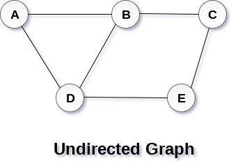
A Graph G(V, E) with 5 vertices (A, B, C, D, E) and six edges ((A,B), (B,C), (C,E), (E,D), (D,B), (D,A)) is shown in the following figure.
Directed and Undirected Graph
A graph can be directed or undirected. However, in an undirected graph, edges are not associated with the directions with them. An undirected graph is shown in the above figure since its edges are not attached with any of the directions. If an edge exists between vertex A and B then the vertices can be traversed from B to A as well as A to B.
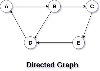
In a directed graph, edges form an ordered pair. Edges represent a specific path from some vertex A to another vertex B. Node A is called initial node while node B is called terminal node.
A directed graph is shown in the following figure.
Graph Terminology
A path can be defined as the sequence of nodes that are followed in order to reach some terminal node V from the initial node U.
A path will be called as closed path if the initial node is same as terminal node. A path will be closed path if V0=VN.
If all the nodes of the graph are distinct with an exception V0=VN, then such path P is called as closed simple path.
A cycle can be defined as the path which has no repeated edges or vertices except the first and last vertices.
A connected graph is the one in which some path exists between every two vertices (u, v) in V. There are no isolated nodes in connected graph.
A complete graph is the one in which every node is connected with all other nodes. A complete graph contain n(n-1)/2 edges where n is the number of nodes in the graph.
In a weighted graph, each edge is assigned with some data such as length or weight. The weight of an edge e can be given as w(e) which must be a positive (+) value indicating the cost of traversing the edge.
A digraph is a directed graph in which each edge of the graph is associated with some direction and the traversing can be done only in the specified direction.
An edge that is associated with the similar end points can be called as Loop.
If two nodes u and v are connected via an edge e, then the nodes u and v are called as neighbours or adjacent nodes.
A degree of a node is the number of edges that are connected with that node. A node with degree 0 is called as isolated node.
Key takeaway
A graph can be defined as group of vertices and edges that are used to connect these vertices. A graph can be seen as a cyclic tree, where the vertices (Nodes) maintain any complex relationship among them instead of having parent child relationship.
A graph G can be defined as an ordered set G(V, E) where V(G) represents the set of vertices and E(G) represents the set of edges which are used to connect these vertices.
By Graph representation, we simply mean the technique which is to be used in order to store some graph into the computer's memory.
There are two ways to store Graph into the computer's memory. In this part of this tutorial, we discuss each one of them in detail.
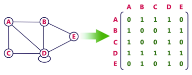
In sequential representation, we use adjacency matrix to store the mapping represented by vertices and edges. In adjacency matrix, the rows and columns are represented by the graph vertices. A graph having n vertices, will have a dimension n x n.
An entry Mij in the adjacency matrix representation of an undirected graph G will be 1 if there exists an edge between Vi and Vj.
An undirected graph and its adjacency matrix representation is shown in the following figure.
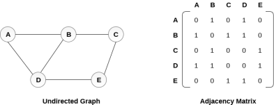
in the above figure, we can see the mapping among the vertices (A, B, C, D, E) is represented by using the adjacency matrix which is also shown in the figure.
There exists different adjacency matrices for the directed and undirected graph. In directed graph, an entry Aij will be 1 only when there is an edge directed from Vi to Vj.
A directed graph and its adjacency matrix representation is shown in the following figure.

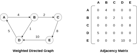
Representation of weighted directed graph is different. Instead of filling the entry by 1, the Non- zero entries of the adjacency matrix are represented by the weight of respective edges.
The weighted directed graph along with the adjacency matrix representation is shown in the following figure.
In the linked representation, an adjacency list is used to store the Graph into the computer's memory.
Consider the undirected graph shown in the following figure and check the adjacency list representation.

An adjacency list is maintained for each node present in the graph which stores the node value and a pointer to the next adjacent node to the respective node. If all the adjacent nodes are traversed then store the NULL in the pointer field of last node of the list. The sum of the lengths of adjacency lists is equal to the twice of the number of edges present in an undirected graph.
Consider the directed graph shown in the following figure and check the adjacency list representation of the graph.
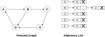
In a directed graph, the sum of lengths of all the adjacency lists is equal to the number of edges present in the graph.
In the case of weighted directed graph, each node contains an extra field that is called the weight of the node. The adjacency list representation of a directed graph is shown in the following figure.

Key takeaway
By Graph representation, we simply mean the technique which is to be used in order to store some graph into the computer's memory.
There are two ways to store Graph into the computer's memory. In this part of this tutorial, we discuss each one of them in detail.
In graph theory, a graph representation is a technique to store graph into the memory of computer.
To represent a graph, we just need the set of vertices, and for each vertex the neighbours of the vertex (vertices which is directly connected to it by an edge). If it is a weighted graph, then the weight will be associated with each edge.
There are different ways to optimally represent a graph, depending on the density of its edges, type of operations to be performed and ease of use.
Consider the following undirected graph representation:
Undirected graph representation
Directed graph representation
See the directed graph representation:
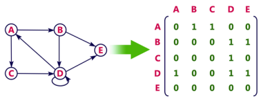
In the above examples, 1 represents an edge from row vertex to column vertex, and 0 represents no edge from row vertex to column vertex.
Undirected weighted graph represenation
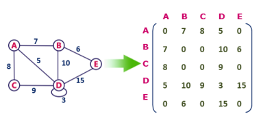
Pros: Representation is easier to implement and follow.
Cons: It takes a lot of space and time to visit all the neighbors of a vertex, we have to traverse all the vertices in the graph, which takes quite some time.
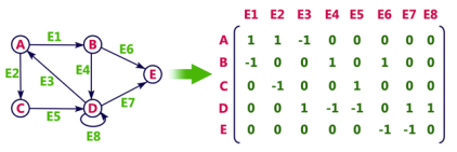
In Incidence matrix representation, graph can be represented using a matrix of size:
Total number of vertices by total number of edges.
It means if a graph has 4 vertices and 6 edges, then it can be represented using a matrix of 4X6 class. In this matrix, columns represent edges and rows represent vertices.
This matrix is filled with either 0 or 1 or -1. Where,
Consider the following directed graph representation.
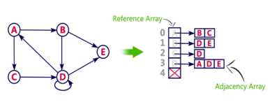
Let's see the following directed graph representation implemented using linked list:

We can also implement this representation using array as follows:
Pros:
Cons:
Key takeaway
In graph theory, a graph representation is a technique to store graph into the memory of computer.
To represent a graph, we just need the set of vertices, and for each vertex the neighbours of the vertex (vertices which is directly connected to it by an edge). If it is a weighted graph, then the weight will be associated with each edge.
There are different ways to optimally represent a graph, depending on the density of its edges, type of operations to be performed and ease of use.
In this part of the tutorial we will discuss the techniques by using which, we can traverse all the vertices of the graph.
Traversing the graph means examining all the nodes and vertices of the graph. There are two standard methods by using which, we can traverse the graphs. Let’s discuss each one of them in detail.
Breadth First Search (BFS) Algorithm
Breadth first search is a graph traversal algorithm that starts traversing the graph from root node and explores all the neighbouring nodes. Then, it selects the nearest node and explore all the unexplored nodes. The algorithm follows the same process for each of the nearest node until it finds the goal.
The algorithm of breadth first search is given below. The algorithm starts with examining the node A and all of its neighbours. In the next step, the neighbours of the nearest node of A are explored and process continues in the further steps. The algorithm explores all neighbours of all the nodes and ensures that each node is visited exactly once and no node is visited twice.
Consider the graph G shown in the following image, calculate the minimum path p from node A to node E. Given that each edge has a length of 1.

Minimum Path P can be found by applying breadth first search algorithm that will begin at node A and will end at E. the algorithm uses two queues, namely QUEUE1 and QUEUE2. QUEUE1 holds all the nodes that are to be processed while QUEUE2 holds all the nodes that are processed and deleted from QUEUE1.
Let’s start examining the graph from Node A.
1. Add A to QUEUE1 and NULL to QUEUE2.
2. Delete the Node A from QUEUE1 and insert all its neighbours. Insert Node A into QUEUE2
3. Delete the node B from QUEUE1 and insert all its neighbours. Insert node B into QUEUE2.
4. Delete the node D from QUEUE1 and insert all its neighbours. Since F is the only neighbour of it which has been inserted, we will not insert it again. Insert node D into QUEUE2.
5. Delete the node C from QUEUE1 and insert all its neighbours. Add node C to QUEUE2.
6. Remove F from QUEUE1 and add all its neighbours. Since all of its neighbours has already been added, we will not add them again. Add node F to QUEUE2.
7. Remove E from QUEUE1, all of E's neighbours has already been added to QUEUE1 therefore we will not add them again. All the nodes are visited and the target node i.e. E is encountered into QUEUE2.
Now, backtrack from E to A, using the nodes available in QUEUE2.
The minimum path will be A → B → C → E.
Depth First Search (DFS) Algorithm
Depth first search (DFS) algorithm starts with the initial node of the graph G, and then goes to deeper and deeper until we find the goal node or the node which has no children. The algorithm, then backtracks from the dead end towards the most recent node that is yet to be completely unexplored.
The data structure which is being used in DFS is stack. The process is similar to BFS algorithm. In DFS, the edges that leads to an unvisited node are called discovery edges while the edges that leads to an already visited node are called block edges.
Consider the graph G along with its adjacency list, given in the figure below. Calculate the order to print all the nodes of the graph starting from node H, by using depth first search (DFS) algorithm.
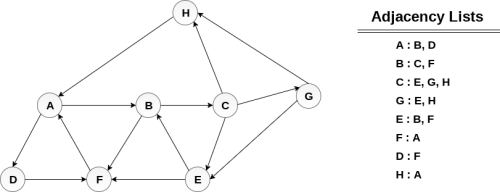
Push H onto the stack
POP the top element of the stack i.e. H, print it and push all the neighbours of H onto the stack that are is ready state.
Pop the top element of the stack i.e. A, print it and push all the neighbours of A onto the stack that are in ready state.
Pop the top element of the stack i.e. D, print it and push all the neighbours of D onto the stack that are in ready state.
Pop the top element of the stack i.e. F, print it and push all the neighbours of F onto the stack that are in ready state.
Pop the top of the stack i.e. B and push all the neighbours
Pop the top of the stack i.e. C and push all the neighbours.
Pop the top of the stack i.e. G and push all its neighbours.
Pop the top of the stack i.e. E and push all its neighbours.
Hence, the stack now becomes empty and all the nodes of the graph have been traversed.
The printing sequence of the graph will be:
Key takeaway
In this part of the tutorial we will discuss the techniques by using which, we can traverse all the vertices of the graph.
Traversing the graph means examining all the nodes and vertices of the graph. There are two standard methods by using which, we can traverse the graphs. Lets discuss each one of them in detail.
Spanning tree can be defined as a sub-graph of connected, undirected graph G that is a tree produced by removing the desired number of edges from a graph. In other words, Spanning tree is a non-cyclic sub-graph of a connected and undirected graph G that connects all the vertices together. A graph G can have multiple spanning trees.
There can be weights assigned to every edge in a weighted graph. However, A minimum spanning tree is a spanning tree which has minimal total weight. In other words, minimum spanning tree is the one which contains the least weight among all other spanning tree of some particular graph.
In this section of the tutorial, we will discuss the algorithms to calculate the shortest path between two nodes in a graph.
There are two algorithms which are being used for this purpose.
• Prim's Algorithm
• Kruskal's Algorithm
Prim's Algorithm is used to find the minimum spanning tree from a graph. Prim's algorithm finds the subset of edges that includes every vertex of the graph such that the sum of the weights of the edges can be minimized.
Prim's algorithm starts with the single node and explore all the adjacent nodes with all the connecting edges at every step. The edges with the minimal weights causing no cycles in the graph got selected.
The algorithm is given as follows.
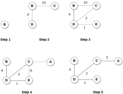
Construct a minimum spanning tree of the graph given in the following figure by using prim's algorithm.
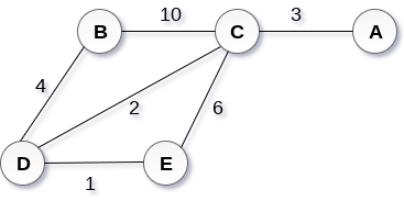
The graph produces in the step 4 is the minimum spanning tree of the graph shown in the above figure.
The cost of MST will be calculated as;
cost(MST) = 4 + 2 + 1 + 3 = 10 units.
Output
0 1 5
0 2 0
0 3 8
1 4 6
Kruskal's Algorithm is used to find the minimum spanning tree for a connected weighted graph. The main target of the algorithm is to find the subset of edges by using which, we can traverse every vertex of the graph. Kruskal's algorithm follows greedy approach which finds an optimum solution at every stage instead of focusing on a global optimum.
The Kruskal's algorithm is given as follows.
ELSE
Discard the edge
Apply the Kruskal's algorithm on the graph given as follows.
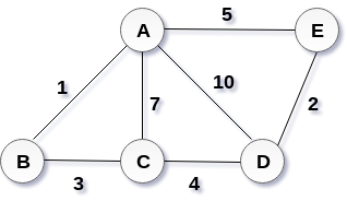
the weight of the edges given as:
Edge | AE | AD | AC | AB | BC | CD | DE |
Weight | 5 | 10 | 7 | 1 | 3 | 4 | 2 |
Sort the edges according to their weights.
Edge | AB | DE | BC | CD | AE | AC | AD |
Weight | 1 | 2 | 3 | 4 | 5 | 7 | 10 |
Start constructing the tree;
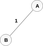
Add AB to the MST;
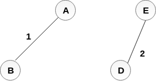
Add DE to the MST;
Add BC to the MST;

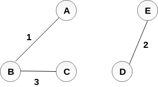
The next step is to add AE, but we can't add that as it will cause a cycle.
The next edge to be added is AC, but it can't be added as it will cause a cycle.
The next edge to be added is AD, but it can't be added as it will contain a cycle.
Hence, the final MST is the one which is shown in the step 4.
the cost of MST = 1 + 2 + 3 + 4 = 10.
Output
Enter Nodes and edges5
5
Enter the value of X, Y and edges5
4
3
Enter the value of X, Y and edges2
3
1
Enter the value of X, Y and edges1
2
3
Enter the value of X, Y and edges5
4
3
Enter the value of X, Y and edges23
3
4
Minimum cost is 11
Key takeaway
Spanning tree can be defined as a sub-graph of connected, undirected graph G that is a tree produced by removing the desired number of edges from a graph. In other words, Spanning tree is a non-cyclic sub-graph of a connected and undirected graph G that connects all the vertices together. A graph G can have multiple spanning trees.
There can be weights assigned to every edge in a weighted graph. However, A minimum spanning tree is a spanning tree which has minimal total weight. In other words, minimum spanning tree is the one which contains the least weight among all other spanning tree of some particular graph.
An algorithm is designed to achieve optimum solution for a given problem. In greedy algorithm approach, decisions are made from the given solution domain. As being greedy, the closest solution that seems to provide an optimum solution is chosen.
Greedy algorithms try to find a localized optimum solution, which may eventually lead to globally optimized solutions. However, generally greedy algorithms do not provide globally optimized solutions.
This problem is to count to a desired value by choosing the least possible coins and the greedy approach forces the algorithm to pick the largest possible coin. If we are provided coins of ₹ 1, 2, 5 and 10 and we are asked to count ₹ 18 then the greedy procedure will be −
Though, it seems to be working fine, for this count we need to pick only 4 coins. But if we slightly change the problem then the same approach may not be able to produce the same optimum result.
For the currency system, where we have coins of 1, 7, 10 value, counting coins for value 18 will be absolutely optimum but for count like 15, it may use more coins than necessary. For example, the greedy approach will use 10 + 1 + 1 + 1 + 1 + 1, total 6 coins. Whereas the same problem could be solved by using only 3 coins (7 + 7 + 1)
Hence, we may conclude that the greedy approach picks an immediate optimized solution and may fail where global optimization is a major concern.
Most networking algorithms use the greedy approach. Here is a list of few of them −
There are lots of similar problems that uses the greedy approach to find an optimum solution.
Key takeaway
An algorithm is designed to achieve optimum solution for a given problem. In greedy algorithm approach, decisions are made from the given solution domain. As being greedy, the closest solution that seems to provide an optimum solution is chosen.
Greedy algorithms try to find a localized optimum solution, which may eventually lead to globally optimized solutions. However, generally greedy algorithms do not provide globally optimized solutions.
It is a greedy algorithm that solves the single-source shortest path problem for a directed graph G = (V, E) with nonnegative edge weights, i.e., w (u, v) ≥ 0 for each edge (u, v) ∈ E.
Dijkstra's Algorithm maintains a set S of vertices whose final shortest - path weights from the source s have already been determined. That's for all vertices v ∈ S; we have d [v] = δ (s, v). The algorithm repeatedly selects the vertex u ∈ V - S with the minimum shortest - path estimate, insert u into S and relaxes all edges leaving u.
Because it always chooses the "lightest" or "closest" vertex in V - S to insert into set S, it is called as the greedy strategy.
Dijkstra's Algorithm (G, w, s)
1. INITIALIZE - SINGLE - SOURCE (G, s)
2. S←∅
3. Q←V [G]
4. while Q ≠ ∅
5. do u ← EXTRACT - MIN (Q)
6. S ← S ∪ {u}
7. for each vertex v ∈ Adj [u]
8. do RELAX (u, v, w)
Analysis: The running time of Dijkstra's algorithm on a graph with edges E and vertices V can be expressed as a function of |E| and |V| using the Big - O notation. The simplest implementation of the Dijkstra's algorithm stores vertices of set Q in an ordinary linked list or array, and operation Extract - Min (Q) is simply a linear search through all vertices in Q. In this case, the running time is O (|V2 |+|E|=O(V2 ).
Example:

Solution:
Step1: Q =[s, t, x, y, z]
We scanned vertices one by one and find out its adjacent. Calculate the distance of each adjacent to the source vertices.
We make a stack, which contains those vertices which are selected after computation of shortest distance.
Firstly we take's' in stack M (which is a source)
Step 2: Now find the adjacent of s that are t and y.
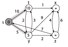
Case - (i) s → t
d [v] > d [u] + w [u, v]
d [t] > d [s] + w [s, t]
∞ > 0 + 10 [false condition]
Then d [t] ← 10
π [t] ← 5
Adj [s] ← t, y
Case - (ii) s→ y
d [v] > d [u] + w [u, v]
d [y] > d [s] + w [s, y]
∞ > 0 + 5 [false condition]
∞ > 5
Then d [y] ← 5
π [y] ← 5
By comparing case (i) and case (ii)
Adj [s] → t = 10, y = 5
y is shortest
y is assigned in 5 = [s, y]
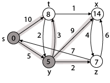
Step 3: Now find the adjacent of y that is t, x, z.
Case - (i) y →t
d [v] > d [u] + w [u, v]
d [t] > d [y] + w [y, t]
10 > 5 + 3
10 > 8
Then d [t] ← 8
π [t] ← y
Case - (ii) y → x
d [v] > d [u] + w [u, v]
d [x] > d [y] + w [y, x]
∞ > 5 + 9
∞ > 14
Then d [x] ← 14
π [x] ← 14
Case - (iii) y → z
d [v] > d [u] + w [u, v]
d [z] > d [y] + w [y, z]
∞ > 5 + 2
∞ > 7
Then d [z] ← 7
π [z] ← y
By comparing case (i), case (ii) and case (iii)
Adj [y] → x = 14, t = 8, z =7
z is shortest
z is assigned in 7 = [s, z]
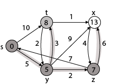
Step - 4 Now we will find adj [z] that are s, x
Case - (i) z → x
d [v] > d [u] + w [u, v]
d [x] > d [z] + w [z, x]
14 > 7 + 6
14 > 13
Then d [x] ← 13
π [x] ← z
Case - (ii) z → s
d [v] > d [u] + w [u, v]
d [s] > d [z] + w [z, s]
0 > 7 + 7
0 > 14
∴ This condition does not satisfy so it will be discarded.
Now we have x = 13.

Step 5: Now we will find Adj [t]
Adj [t] → [x, y] [Here t is u and x and y are v]
Case - (i) t → x
d [v] > d [u] + w [u, v]
d [x] > d [t] + w [t, x]
13 > 8 + 1
13 > 9
Then d [x] ← 9
π [x] ← t
Case - (ii) t → y
d [v] > d [u] + w [u, v]
d [y] > d [t] + w [t, y]
5 > 10
∴ This condition does not satisfy so it will be discarded.
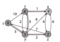
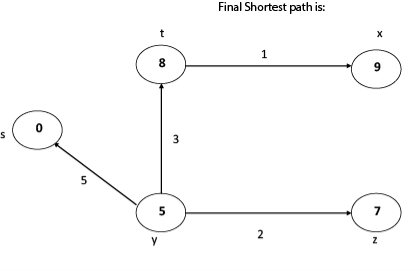
Thus we get all shortest path vertex as
Weight from s to y is 5
Weight from s to z is 7
Weight from s to t is 8
Weight from s to x is 9
These are the shortest distance from the source's' in the given graph.
Disadvantage of Dijkstra's Algorithm:
Key takeaway
It is a greedy algorithm that solves the single-source shortest path problem for a directed graph G = (V, E) with nonnegative edge weights, i.e., w (u, v) ≥ 0 for each edge (u, v) ∈ E.
Dijkstra's Algorithm maintains a set S of vertices whose final shortest - path weights from the source s have already been determined. That's for all vertices v ∈ S; we have d [v] = δ (s, v). The algorithm repeatedly selects the vertex u ∈ V - S with the minimum shortest - path estimate, insert u into S and relaxes all edges leaving u.
Because it always chooses the "lightest" or "closest" vertex in V - S to insert into set S, it is called as the greedy strategy.
It aims to figure out the shortest path from each vertex v to every other u. Storing all the paths explicitly can be very memory expensive indeed, as we need one spanning tree for each vertex. This is often impractical regarding memory consumption, so these are generally considered as all pairs-shortest distance problems, which aim to find just the distance from each to each node to another. We usually want the output in tabular form: the entry in u's row and v's column should be the weight of the shortest path from u to v.
Three approaches for improvement:
Algorithm | Cost |
Matrix Multiplication | O (V3 logV) |
Floyd-Warshall | O (V3) |
Johnson O | (V2 log?V+VE) |
Unlike the single-source algorithms, which assume an adjacency list representation of the graph, most of the algorithm uses an adjacency matrix representation. (Johnson's Algorithm for sparse graphs uses adjacency lists.) The input is a n x n matrix W representing the edge weights of an n-vertex directed graph G = (V, E). That is, W = (wij), where

Let the vertices of G be V = {1, 2........n} and consider a subset {1, 2........k} of vertices for some k. For any pair of vertices i, j ∈ V, considered all paths from i to j whose intermediate vertices are all drawn from {1, 2.......k}, and let p be a minimum weight path from amongst them. The Floyd-Warshall algorithm exploits a link between path p and shortest paths from i to j with all intermediate vertices in the set {1, 2.......k-1}. The link depends on whether or not k is an intermediate vertex of path p.
If k is not an intermediate vertex of path p, then all intermediate vertices of path p are in the set {1, 2........k-1}. Thus, the shortest path from vertex i to vertex j with all intermediate vertices in the set {1, 2.......k-1} is also the shortest path i to j with all intermediate vertices in the set {1, 2.......k}.
If k is an intermediate vertex of path p, then we break p down into i → k → j.
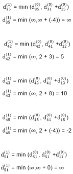
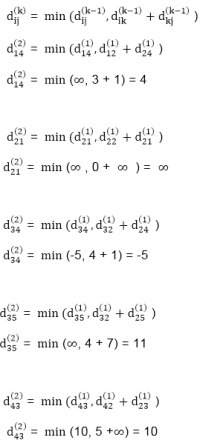
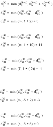
Let dij(k) be the weight of the shortest path from vertex i to vertex j with all intermediate vertices in the set {1, 2.......k}.
A recursive definition is given by

FLOYD - WARSHALL (W)
1. n ← rows [W].
2. D0 ← W
3. for k ← 1 to n
4. do for i ← 1 to n
5. do for j ← 1 to n
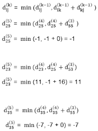
6. do dij(k) ← min (dij(k-1),dik(k-1)+dkj(k-1) )
7. return D(n)
The strategy adopted by the Floyd-Warshall algorithm is Dynamic Programming. The running time of the Floyd-Warshall algorithm is determined by the triply nested for loops of lines 3-6. Each execution of line 6 takes O (1) time. The algorithm thus runs in time θ(n3 ).
Example: Apply Floyd-Warshall algorithm for constructing the shortest path. Show that matrices D(k) and π(k) computed by the Floyd-Warshall algorithm for the graph.
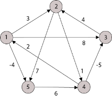
Solution:

Step (i) When k = 0

Step (ii) When k =1
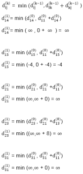

Step (iii) When k = 2

Step (iv) When k = 3


Step (v) When k = 4
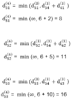

Step (vi) When k = 5

TRANSITIVE- CLOSURE (G)
1. n ← |V[G]|
2. for i ← 1 to n
3. do for j ← 1 to n
4. do if i = j or (i, j) ∈ E [G]
5. the  ← 1
← 1
6. else  ← 0
← 0
7. for k ← 1 to n
8. do for i ← 1 to n
9. do for j ← 1 to n
10. dod ij(k) ← 
11. Return T(n).
The problem is to find the shortest path between every pair of vertices in a given weighted directed graph and weight may be negative. Using Johnson's Algorithm, we can find all pairs shortest path in O (V2 log? V+VE) time. Johnson's Algorithm uses both Dijkstra's Algorithm and Bellman-Ford Algorithm.
Johnson's Algorithm uses the technique of "reweighting." If all edge weights w in a graph G = (V, E) are nonnegative, we can find the shortest paths between all pairs of vertices by running Dijkstra's Algorithm once from each vertex. If G has negative - weight edges, we compute a new - set of non - negative edge weights that allows us to use the same method. The new set of edges weight w must satisfy two essential properties:
Given a weighted, directed graph G = (V, E) with weight function w: E→R and let h: v→R be any function mapping vertices to a real number.
For each edge (u, v) ∈ E define

Where h (u) = label of u
h (v) = label of v
JOHNSON (G)
1. Compute G' where V [G'] = V[G] ∪ {S} and
E [G'] = E [G] ∪ {(s, v): v ∈ V [G]}
2. If BELLMAN-FORD (G',w, s) = FALSE
then "input graph contains a negative weight cycle"
else
for each vertex v ∈ V [G']
do h (v) ← δ(s, v)
Computed by Bellman-Ford algorithm
for each edge (u, v) ∈ E[G']
do w (u, v) ← w (u, v) + h (u) - h (v)
for each edge u ∈ V [G]
do run DIJKSTRA (G, w, u) to compute
δ (u, v) for all v ∈ V [G]
for each vertex v ∈ V [G]
do duv← δ (u, v) + h (v) - h (u)
Return D.
Example:
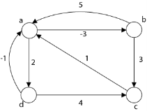
Step1: Take any source vertex's' outside the graph and make distance from's' to every vertex '0'.
Step2: Apply Bellman-Ford Algorithm and calculate minimum weight on each vertex.
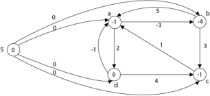
Step3: w (a, b) = w (a, b) + h (a) - h (b)
= -3 + (-1) - (-4)
= 0
w (b, a) = w (b, a) + h (b) - h (a)
= 5 + (-4) - (-1)
= 2
w (b, c) = w (b, c) + h (b) - h (c)
w (b, c) = 3 + (-4) - (-1)
= 0
w (c, a) = w (c, a) + h (c) - h (a)
w (c, a) = 1 + (-1) - (-1)
= 1
w (d, c) = w (d, c) + h (d) - h (c)
w (d, c) = 4 + 0 - (-1)
= 5
w (d, a) = w (d, a) + h (d) - h (a)
w (d, a) = -1 + 0 - (-1)
= 0
w (a, d) = w (a, d) + h (a) - h (d)
w (a, d) = 2 + (-1) - 0 = 1
Step 4: Now all edge weights are positive and now we can apply Dijkstra's Algorithm on each vertex and make a matrix corresponds to each vertex in a graph
Case 1: 'a' as a source vertex
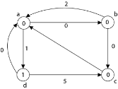

Case 2: 'b' as a source vertex
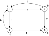

Case 3: 'c' as a source vertex
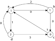

Case4:'d' as source vertex
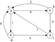


Step5:
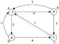
duv ← δ (u, v) + h (v) - h (u)
d (a, a) = 0 + (-1) - (-1) = 0
d (a, b) = 0 + (-4) - (-1) = -3
d (a, c) = 0 + (-1) - (-1) = 0
d (a, d) = 1 + (0) - (-1) = 2
d (b, a) = 1 + (-1) - (-4) = 4
d (b, b) = 0 + (-4) - (-4) = 0
d (c, a) = 1 + (-1) - (-1) = 1
d (c, b) = 1 + (-4) - (-1) = -2
d (c, c) = 0
d (c, d) = 2 + (0) - (-1) = 3
d (d, a) = 0 + (-1) - (0) = -1
d (d, b) = 0 + (-4) - (0) = -4
d (d, c) = 0 + (-1) - (0) = -1
d (d, d) = 0

Key takeaway
It aims to figure out the shortest path from each vertex v to every other u. Storing all the paths explicitly can be very memory expensive indeed, as we need one spanning tree for each vertex. This is often impractical regarding memory consumption, so these are generally considered as all pairs-shortest distance problems, which aim to find just the distance from each to each node to another. We usually want the output in tabular form: the entry in u's row and v's column should be the weight of the shortest path from u to v.
References:
1. Horowitz, Sahani, Dinesh Mehata, ―Fundamentals of Data Structures in C++‖, Galgotia Publisher, ISBN: 8175152788, 9788175152786.
2. M Folk, B Zoellick, G. Riccardi, ―File Structures‖, Pearson Education, ISBN:81-7758-37-5
3. Peter Brass, ―Advanced Data Structures‖, Cambridge University Press, ISBN: 978-1-107- 43982-5
4. A. Aho, J. Hopcroft, J. Ulman, ―Data Structures and Algorithms‖, Pearson Education, 1998, ISBN-0-201-43578-0.
5. Michael J Folk, ―File Structures an Object-Oriented Approach with C++‖, Pearson Education, ISBN: 81-7758-373-5.
6. Sartaj Sahani, ―Data Structures, Algorithms and Applications in C++‖, Second Edition, University Press, ISBN:81-7371522 X.
7. G A V Pai, ―Data Structures and Algorithms‖, The McGraw-Hill Companies, ISBN - 9780070667266.
8. Goodrich, Tamassia, Goldwasser, ―Data Structures and Algorithms in Java‖, Wiley Publication, ISBN: 9788126551903