Search Trees
Symbol table is an important data structure created and maintained by compilers in order to store information about the occurrence of various entities such as variable names, function names, objects, classes, interfaces, etc. Symbol table is used by both the analysis and the synthesis parts of a compiler.
A symbol table may serve the following purposes depending upon the language in hand:
A symbol table is simply a table which can be either linear or a hash table. It maintains an entry for each name in the following format:
<symbol name, type, attribute>
For example, if a symbol table has to store information about the following variable declaration:
static int interest;
then it should store the entry such as:
<interest, int, static>
The attribute clause contains the entries related to the name.
If a compiler is to handle a small amount of data, then the symbol table can be implemented as an unordered list, which is easy to code, but it is only suitable for small tables only. A symbol table can be implemented in one of the following ways:
Among all, symbol tables are mostly implemented as hash tables, where the source code symbol itself is treated as a key for the hash function and the return value is the information about the symbol.
A symbol table, either linear or hash, should provide the following operations.
This operation is more frequently used by analysis phase, i.e., the first half of the compiler where tokens are identified and names are stored in the table. This operation is used to add information in the symbol table about unique names occurring in the source code. The format or structure in which the names are stored depends upon the compiler in hand.
An attribute for a symbol in the source code is the information associated with that symbol. This information contains the value, state, scope, and type about the symbol. The insert() function takes the symbol and its attributes as arguments and stores the information in the symbol table.
For example:
int a;
should be processed by the compiler as:
insert(a, int);
lookup() operation is used to search a name in the symbol table to determine:
The format of lookup() function varies according to the programming language. The basic format should match the following:
lookup(symbol)
This method returns 0 (zero) if the symbol does not exist in the symbol table. If the symbol exists in the symbol table, it returns its attributes stored in the table.
A compiler maintains two types of symbol tables: a global symbol table which can be accessed by all the procedures and scope symbol tables that are created for each scope in the program.
To determine the scope of a name, symbol tables are arranged in hierarchical structure as shown in the example below:
. . .
int value=10;
void pro_one()
{
int one_1;
int one_2;
{ \
int one_3; |_ inner scope 1
int one_4; |
} /
int one_5;
{ \
int one_6; |_ inner scope 2
int one_7; |
} /
}
void pro_two()
{
int two_1;
int two_2;
{ \
int two_3; |_ inner scope 3
int two_4; |
} /
int two_5;
}
. . .
The above program can be represented in a hierarchical structure of symbol tables:
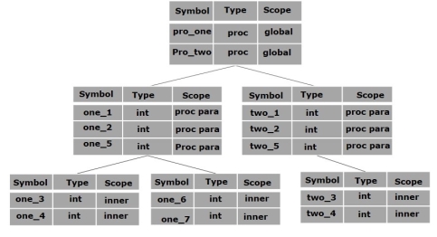
The global symbol table contains names for one global variable (int value) and two procedure names, which should be available to all the child nodes shown above. The names mentioned in the pro_one symbol table (and all its child tables) are not available for pro_two symbols and its child tables.
This symbol table data structure hierarchy is stored in the semantic analyzer and whenever a name needs to be searched in a symbol table, it is searched using the following algorithm:
Key takeaway
Symbol table is an important data structure created and maintained by compilers in order to store information about the occurrence of various entities such as variable names, function names, objects, classes, interfaces, etc. Symbol table is used by both the analysis and the synthesis parts of a compiler.
A symbol table may serve the following purposes depending upon the language in hand:
Data Structure is a way of storing and organising data efficiently such that the required operations on them can be performed be efficient with respect to time as well as memory. Simply, Data Structure are used to reduce complexity (mostly the time complexity) of the code.
Data structures can be two types:
1. Static Data Structure
2. Dynamic Data Structure
What is a Static Data structure?
In Static data structure the size of the structure is fixed. The content of the data structure can be modified but without changing the memory space allocated to it.

Example of Static Data Structures: Array
What is Dynamic Data Structure?
In Dynamic data structure the size of the structure in not fixed and can be modified during the operations performed on it. Dynamic data structures are designed to facilitate change of data structures in the run time.

Example of Dynamic Data Structures: Linked List
Static Data Structure vs Dynamic Data Structure
Static Data structure has fixed memory size whereas in Dynamic Data Structure, the size can be randomly updated during run time which may be considered efficient with respect to memory complexity of the code. Static Data Structure provides more easier access to elements with respect to dynamic data structure. Unlike static data structures, dynamic data structures are flexible.
Use of Dynamic Data Structure in Competitive Programming
In competitive programming the constraints on memory limit is not much high and we cannot exceed the memory limit. Given higher value of the constraints we cannot allocate a static data structure of that size so Dynamic Data Structures can be useful.
Key takeaway
Data Structure is a way of storing and organising data efficiently such that the required operations on them can be performed be efficient with respect to time as well as memory. Simply, Data Structure are used to reduce complexity (mostly the time complexity) of the code.
Data structures can be two types:
1. Static Data Structure
2. Dynamic Data Structure
A weight-balanced binary tree is a binary tree which is balanced based on knowledge of the probabilities of searching for each individual node. Within each subtree, the node with the highest weight appears at the root. This can result in more efficient searching performance. Construction of such a tree is similar to that of a Treap, but node weights are chosen randomly in the latter.
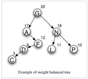
Example of weight balanced tree
The diagram
In the diagram to the right, the letters represent node values and the numbers represent node weights. Values are used to order the tree, as in a general binary search tree. The weight may be thought of as a probability or activity count associated with the node. In the diagram, the root is G because its weight is the greatest in the tree. The left subtree begins with A because, out of all nodes with values that come before G, A has the highest weight. Similarly, N is the highest-weighted node that comes after G.
Timing analysis
A weight balanced tree gives close to optimal values for the expected length of successful search calculations. From the above example we get
ELOSS = depth(node A)*probability(node A) + depth(node C)
*probability(node C) + ... ELOSS = 2*0.17 + 5*0.03 + 4*0.09 + 3*0.12 + 1*0.20 + 3*0.11 + 3*0.10 + 2*0.18 ELOSS = 2.4
This is the expected number of nodes that will be examined before finding the desired node.
Key takeaway
A weight-balanced binary tree is a binary tree which is balanced based on knowledge of the probabilities of searching for each individual node. Within each subtree, the node with the highest weight appears at the root. This can result in more efficient searching performance. Construction of such a tree is similar to that of a Treap, but node weights are chosen randomly in the latter.
A set of integers are given in the sorted order and another array freq to frequency count. Our task is to create a binary search tree with those data to find minimum cost for all searches.
An auxiliary array cost[n, n] is created to solve and store the solution of sub problems. Cost matrix will hold the data to solve the problem in bottom up manner.
Input − The key values as node and the frequency.
Keys = {10, 12, 20}
Frequency = {34, 8, 50}
Output − The minimum cost is 142.

These are possible BST from the given values.
For case 1, the cost is: (34*1) + (8*2) + (50*3) = 200
For case 2, the cost is: (8*1) + (34*2) + (50*2) = 176.
Similarly, for case 5, the cost is: (50*1) + (34 * 2) + (8 * 3) = 142 (Minimum)
optCostBst(keys, freq, n)
Input: Keys to insert in BST, frequency for each keys, number of keys.
Output: Minimum cost to make optimal BST.
Begin
define cost matrix of size n x n
for i in range 0 to n-1, do
cost[i, i] := freq[i]
done
for length in range 2 to n, do
for i in range 0 to (n-length+1), do
j := i + length – 1
cost[i, j] := ∞
for r in range i to j, done
if r > i, then
c := cost[i, r-1]
else
c := 0
if r < j, then
c := c + cost[r+1, j]
c := c + sum of frequency from i to j
if c < cost[i, j], then
cost[i, j] := c
done
done
done
return cost[0, n-1]
End
#include <iostream>
using namespace std;
int sum(int freq[], int low, int high){ //sum of frequency from low to high range
int sum = 0;
for (int k = low; k <=high; k++)
sum += freq[k];
return sum;
}
int minCostBST(int keys[], int freq[], int n){
int cost[n][n];
for (int i = 0; i < n; i++) //when only one key, move along diagonal elements
cost[i][i] = freq[i];
for (int length=2; length<=n; length++){
for (int i=0; i<=n-length+1; i++){ //from 0th row to n-length+1 row as i
int j = i+length-1;
cost[i][j] = INT_MAX; //initially store to infinity
for (int r=i; r<=j; r++){
//find cost when r is root of subtree
int c = ((r > i)?cost[i][r-1]:0)+((r < j)?cost[r+1][j]:0)+sum(freq, i, j);
if (c < cost[i][j])
cost[i][j] = c;
}
}
}
return cost[0][n-1];
}
int main(){
int keys[] = {10, 12, 20};
int freq[] = {34, 8, 50};
int n = 3;
cout << "Cost of Optimal BST is: "<< minCostBST(keys, freq, n);
}
Cost of Optimal BST is: 142
A Binary Search Tree (BST) is a tree where the key values are stored in the internal nodes. The external nodes are null nodes. The keys are ordered lexicographically, i.e. for each internal node all the keys in the left sub-tree are less than the keys in the node, and all the keys in the right sub-tree are greater.
When we know the frequency of searching each one of the keys, it is quite easy to compute the expected cost of accessing each node in the tree. An optimal binary search tree is a BST, which has minimal expected cost of locating each node
Search time of an element in a BST is O(n), whereas in a Balanced-BST search time is O(log n). Again the search time can be improved in Optimal Cost Binary Search Tree, placing the most frequently used data in the root and closer to the root element, while placing the least frequently used data near leaves and in leaves.
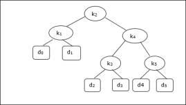
Here, the Optimal Binary Search Tree Algorithm is presented. First, we build a BST from a set of provided n number of distinct keys < k1, k2, k3, ... kn >. Here we assume, the probability of accessing a key Ki is pi. Some dummy keys (d0, d1, d2, ... dn) are added as some searches may be performed for the values which are not present in the Key set K. We assume, for each dummy key di probability of access is qi.
Optimal-Binary-Search-Tree(p, q, n)
e[1…n + 1, 0…n],
w[1…n + 1, 0…n],
root[1…n + 1, 0…n]
for i = 1 to n + 1 do
e[i, i - 1] := qi - 1
w[i, i - 1] := qi - 1
for l = 1 to n do
for i = 1 to n – l + 1 do
j = i + l – 1 e[i, j] := ∞
w[i, i] := w[i, i -1] + pj + qj
for r = i to j do
t := e[i, r - 1] + e[r + 1, j] + w[i, j]
if t < e[i, j]
e[i, j] := t
root[i, j] := r
return e and root
The algorithm requires O (n3) time, since three nested for loops are used. Each of these loops takes on at most n values.
Considering the following tree, the cost is 2.80, though this is not an optimal result.
Node | Depth | Probability | Contribution |
k1 | 1 | 0.15 | 0.30 |
k2 | 0 | 0.10 | 0.10 |
k3 | 2 | 0.05 | 0.15 |
k4 | 1 | 0.10 | 0.20 |
k5 | 2 | 0.20 | 0.60 |
d0 | 2 | 0.05 | 0.15 |
d1 | 2 | 0.10 | 0.30 |
d2 | 3 | 0.05 | 0.20 |
d3 | 3 | 0.05 | 0.20 |
d4 | 3 | 0.05 | 0.20 |
d5 | 3 | 0.10 | 0.40 |
Total |
|
| 2.80 |
To get an optimal solution, using the algorithm discussed in this chapter, the following tables are generated.
In the following tables, column index is i and row index is j.
e | 1 | 2 | 3 | 4 | 5 | 6 |
5 | 2.75 | 2.00 | 1.30 | 0.90 | 0.50 | 0.10 |
4 | 1.75 | 1.20 | 0.60 | 0.30 | 0.05 |
|
3 | 1.25 | 0.70 | 0.25 | 0.05 |
|
|
2 | 0.90 | 0.40 | 0.05 |
|
|
|
1 | 0.45 | 0.10 |
|
|
|
|
0 | 0.05 |
|
|
|
|
|
w | 1 | 2 | 3 | 4 | 5 | 6 |
5 | 1.00 | 0.80 | 0.60 | 0.50 | 0.35 | 0.10 |
4 | 0.70 | 0.50 | 0.30 | 0.20 | 0.05 |
|
3 | 0.55 | 0.35 | 0.15 | 0.05 |
|
|
2 | 0.45 | 0.25 | 0.05 |
|
|
|
1 | 0.30 | 0.10 |
|
|
|
|
0 | 0.05 |
|
|
|
|
|
root | 1 | 2 | 3 | 4 | 5 |
5 | 2 | 4 | 5 | 5 | 5 |
4 | 2 | 2 | 4 | 4 |
|
3 | 2 | 2 | 3 |
|
|
2 | 1 | 2 |
|
|
|
1 | 1 |
|
|
|
|
From these tables, the optimal tree can be formed.
Key takeaway
A set of integers are given in the sorted order and another array freq to frequency count. Our task is to create a binary search tree with those data to find minimum cost for all searches.
An auxiliary array cost[n, n] is created to solve and store the solution of sub problems. Cost matrix will hold the data to solve the problem in bottom up manner.
AVL Tree is invented by GM Adelson - Velsky and EM Landis in 1962. The tree is named AVL in honour of its inventors.
AVL Tree can be defined as height balanced binary search tree in which each node is associated with a balance factor which is calculated by subtracting the height of its right sub-tree from that of its left sub-tree.
Tree is said to be balanced if balance factor of each node is in between -1 to 1, otherwise, the tree will be unbalanced and need to be balanced.
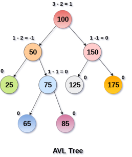
Balance Factor (k) = height (left(k)) - height (right(k))
If balance factor of any node is 1, it means that the left sub-tree is one level higher than the right sub-tree.
If balance factor of any node is 0, it means that the left sub-tree and right sub-tree contain equal height.
If balance factor of any node is -1, it means that the left sub-tree is one level lower than the right sub-tree.
An AVL tree is given in the following figure. We can see that, balance factor associated with each node is in between -1 and +1. therefore, it is an example of AVL tree.
Algorithm | Average case | Worst case |
Space | o(n) | o(n) |
Search | o(log n) | o(log n) |
Insert | o(log n) | o(log n) |
Delete | o(log n) | o(log n) |
Due to the fact that, AVL tree is also a binary search tree therefore, all the operations are performed in the same way as they are performed in a binary search tree. Searching and traversing do not lead to the violation in property of AVL tree. However, insertion and deletion are the operations which can violate this property and therefore, they need to be revisited.
SN | Operation | Description |
1 | Insertion | Insertion in AVL tree is performed in the same way as it is performed in a binary search tree. However, it may lead to violation in the AVL tree property and therefore the tree may need balancing. The tree can be balanced by applying rotations. |
2 | Deletion | Deletion can also be performed in the same way as it is performed in a binary search tree. Deletion may also disturb the balance of the tree therefore; various types of rotations are used to rebalance the tree. |
AVL tree controls the height of the binary search tree by not letting it to be skewed. The time taken for all operations in a binary search tree of height h is O(h). However, it can be extended to O(n) if the BST becomes skewed (i.e. worst case). By limiting this height to log n, AVL tree imposes an upper bound on each operation to be O(log n) where n is the number of nodes.
We perform rotation in AVL tree only in case if Balance Factor is other than -1, 0, and 1. There are basically four types of rotations which are as follows:
Where node A is the node whose balance Factor is other than -1, 0, 1.
The first two rotations LL and RR are single rotations and the next two rotations LR and RL are double rotations. For a tree to be unbalanced, minimum height must be at least 2, Let us understand each rotation
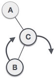
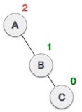
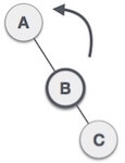
When BST becomes unbalanced, due to a node is inserted into the right subtree of the right subtree of A, then we perform RR rotation, RR rotation is an anticlockwise rotation, which is applied on the edge below a node having balance factor -2
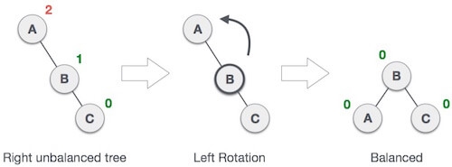
In above example, node A has balance factor -2 because a node C is inserted in the right subtree of A right subtree. We perform the RR rotation on the edge below A.
When BST becomes unbalanced, due to a node is inserted into the left subtree of the left subtree of C, then we perform LL rotation, LL rotation is clockwise rotation, which is applied on the edge below a node having balance factor 2.
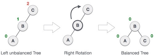
In above example, node C has balance factor 2 because a node A is inserted in the left subtree of C left subtree. We perform the LL rotation on the edge below A.
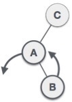
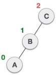
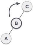
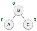
Double rotations are bit tougher than single rotation which has already explained above. LR rotation = RR rotation + LL rotation, i.e., first RR rotation is performed on subtree and then LL rotation is performed on full tree, by full tree we mean the first node from the path of inserted node whose balance factor is other than -1, 0, or 1.
Let us understand each and every step very clearly:
State | Action |
| A node B has been inserted into the right subtree of A the left subtree of C, because of which C has become an unbalanced node having balance factor 2. This case is L R rotation where: Inserted node is in the right subtree of left subtree of C |
| As LR rotation = RR + LL rotation, hence RR (anticlockwise) on subtree rooted at A is performed first. By doing RR rotation, node A, has become the left subtree of B. |
| After performing RR rotation, node C is still unbalanced, i.e., having balance factor 2, as inserted node A is in the left of left of C |
| Now we perform LL clockwise rotation on full tree, i.e. on node C. node C has now become the right subtree of node B, A is left subtree of B |
| Balance factor of each node is now either -1, 0, or 1, i.e. BST is balanced now. |
As already discussed, that double rotations are bit tougher than single rotation which has already explained above. R L rotation = LL rotation + RR rotation, i.e., first LL rotation is performed on subtree and then RR rotation is performed on full tree, by full tree we mean the first node from the path of inserted node whose balance factor is other than -1, 0, or 1.
State | Action |
| A node B has been inserted into the left subtree of C the right subtree of A, because of which A has become an unbalanced node having balance factor - 2. This case is RL rotation where: Inserted node is in the left subtree of right subtree of A |
| As RL rotation = LL rotation + RR rotation, hence, LL (clockwise) on subtree rooted at C is performed first. By doing RR rotation, node C has become the right subtree of B. |
| After performing LL rotation, node A is still unbalanced, i.e. having balance factor -2, which is because of the right-subtree of the right-subtree node A. |
| Now we perform RR rotation (anticlockwise rotation) on full tree, i.e. on node A. node C has now become the right subtree of node B, and node A has become the left subtree of B. |
| Balance factor of each node is now either -1, 0, or 1, i.e., BST is balanced now. |
Q: Construct an AVL tree having the following elements
H, I, J, B, A, E, C, F, D, G, K, L
1. Insert H, I, J
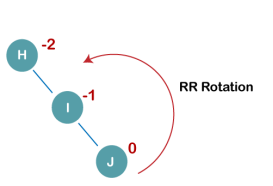
On inserting the above elements, especially in the case of H, the BST becomes unbalanced as the Balance Factor of H is -2. Since the BST is right-skewed, we will perform RR Rotation on node H.
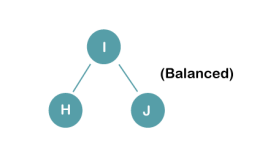
The resultant balance tree is:
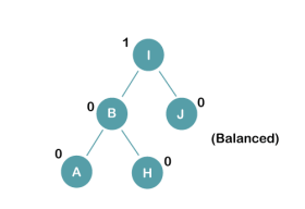
2. Insert B, A
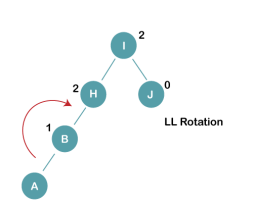
On inserting the above elements, especially in case of A, the BST becomes unbalanced as the Balance Factor of H and I is 2, we consider the first node from the last inserted node i.e. H. Since the BST from H is left-skewed, we will perform LL Rotation on node H.
The resultant balance tree is:
3. Insert E
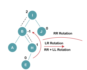
On inserting E, BST becomes unbalanced as the Balance Factor of I is 2, since if we travel from E to I we find that it is inserted in the left subtree of right subtree of I, we will perform LR Rotation on node I. LR = RR + LL rotation
3 a) We first perform RR rotation on node B
The resultant tree after RR rotation is:
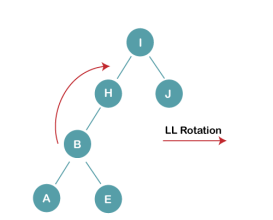
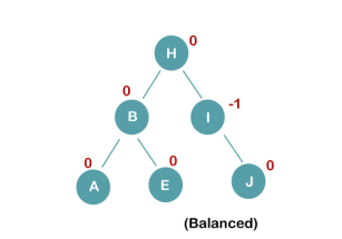
3b) We first perform LL rotation on the node I
The resultant balanced tree after LL rotation is:
4. Insert C, F, D
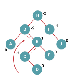
On inserting C, F, D, BST becomes unbalanced as the Balance Factor of B and H is -2, since if we travel from D to B we find that it is inserted in the right subtree of left subtree of B, we will perform RL Rotation on node I. RL = LL + RR rotation.
4a) We first perform LL rotation on node E
The resultant tree after LL rotation is:
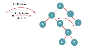
4b) We then perform RR rotation on node B
The resultant balanced tree after RR rotation is:
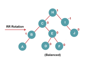
5. Insert G
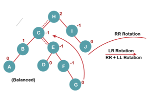
On inserting G, BST become unbalanced as the Balance Factor of H is 2, since if we travel from G to H, we find that it is inserted in the left subtree of right subtree of H, we will perform LR Rotation on node I. LR = RR + LL rotation.
5 a) We first perform RR rotation on node C
The resultant tree after RR rotation is:
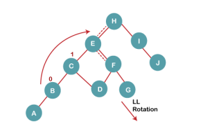
5 b) We then perform LL rotation on node H
The resultant balanced tree after LL rotation is:
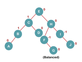
6. Insert K
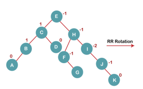
On inserting K, BST becomes unbalanced as the Balance Factor of I is -2. Since the BST is right-skewed from I to K, hence we will perform RR Rotation on the node I.
The resultant balanced tree after RR rotation is:
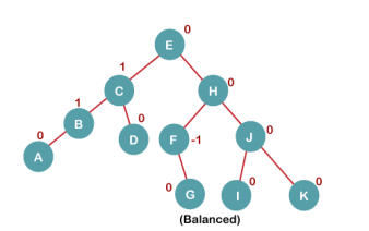
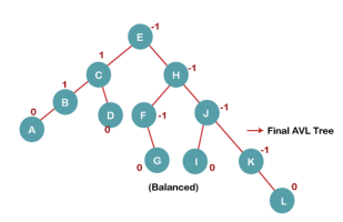
7. Insert L
On inserting the L tree is still balanced as the Balance Factor of each node is now either, -1, 0, +1. Hence the tree is a Balanced AVL tree
A Red Black Tree is a category of the self-balancing binary search tree. It was created in 1972 by Rudolf Bayer who termed them "symmetric binary B-trees."
A red-black tree is a Binary tree where a particular node has color as an extra attribute, either red or black. By check the node colors on any simple path from the root to a leaf, red-black trees secure that no such path is higher than twice as long as any other so that the tree is generally balanced.
A red-black tree must satisfy these properties:
A tree T is an almost red-black tree (ARB tree) if the root is red, but other conditions above hold.
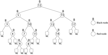
The search-tree operations TREE-INSERT and TREE-DELETE, when runs on a red-black tree with n keys, take O (log n) time. Because they customize the tree, the conclusion may violate the red-black properties. To restore these properties, we must change the color of some of the nodes in the tree and also change the pointer structure.
Restructuring operations on red-black trees can generally be expressed more clearly in details of the rotation operation.

Clearly, the order (Ax By C) is preserved by the rotation operation. Therefore, if we start with a BST and only restructure using rotation, then we will still have a BST i.e. rotation do not break the BST-Property.
LEFT ROTATE (T, x)
1. y ← right [x]
1. y ← right [x]
2. right [x] ← left [y]
3. p [left[y]] ← x
4. p[y] ← p[x]
5. If p[x] = nil [T]
then root [T] ← y
else if x = left [p[x]]
then left [p[x]] ← y
else right [p[x]] ← y
6. left [y] ← x.
7. p [x] ← y.
Example: Draw the complete binary tree of height 3 on the keys {1, 2, 3... 15}. Add the NIL leaves and color the nodes in three different ways such that the black heights of the resulting trees are: 2, 3 and 4.
Solution:
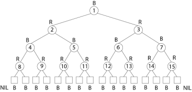
Tree with black-height-2
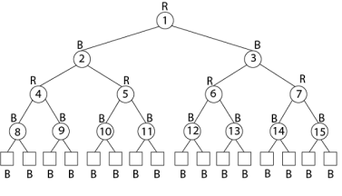
Tree with black-height-3
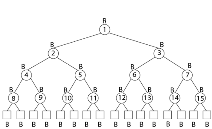
Tree with black-height-4
A discrepancy can decision from a parent and a child both having a red color. This type of discrepancy is determined by the location of the node concerning grandparent, and the color of the sibling of the parent.
RB-INSERT (T, z)
1. y ← nil [T]
2. x ← root [T]
3. while x ≠ NIL [T]
4. do y ← x
5. if key [z] < key [x]
6. then x ← left [x]
7. else x ← right [x]
8. p [z] ← y
9. if y = nil [T]
10. then root [T] ← z
11. else if key [z] < key [y]
12. then left [y] ← z
13. else right [y] ← z
14. left [z] ← nil [T]
15. right [z] ← nil [T]
16. color [z] ← RED
17. RB-INSERT-FIXUP (T, z)
After the insert new node, Coloring this new node into black may violate the black-height conditions and coloring this new node into red may violate coloring conditions i.e. root is black and red node has no red children. We know the black-height violations are hard. So we color the node red. After this, if there is any color violation, then we have to correct them by an RB-INSERT-FIXUP procedure.
RB-INSERT-FIXUP (T, z)
1. while color [p[z]] = RED
2. do if p [z] = left [p[p[z]]]
3. then y ← right [p[p[z]]]
4. If color [y] = RED
5. then color [p[z]] ← BLACK //Case 1
6. color [y] ← BLACK //Case 1
7. color [p[z]] ← RED //Case 1
8. z ← p[p[z]] //Case 1
9. else if z= right [p[z]]
10. then z ← p [z] //Case 2
11. LEFT-ROTATE (T, z) //Case 2
12. color [p[z]] ← BLACK //Case 3
13. color [p [p[z]]] ← RED //Case 3
14. RIGHT-ROTATE (T,p [p[z]]) //Case 3
15. else (same as then clause)
With "right" and "left" exchanged
16. color [root[T]] ← BLACK
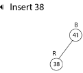
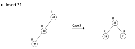
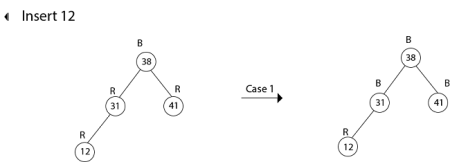
Example: Show the red-black trees that result after successively inserting the keys 41,38,31,12,19,8 into an initially empty red-black tree.
Solution:
Insert 41

Insert 19
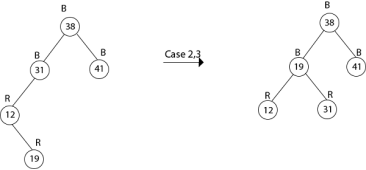
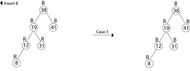
Thus the final tree is
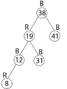
First, search for an element to be deleted
- The replacing node is red, in which case we merely color it black to make up for the loss of one black node.
- The replacing node is black.
The strategy RB-DELETE is a minor change of the TREE-DELETE procedure. After splicing out a node, it calls an auxiliary procedure RB-DELETE-FIXUP that changes colors and performs rotation to restore the red-black properties.
RB-DELETE (T, z)
1. if left [z] = nil [T] or right [z] = nil [T]
2. then y ← z
3. else y ← TREE-SUCCESSOR (z)
4. if left [y] ≠ nil [T]
5. then x ← left [y]
6. else x ← right [y]
7. p [x] ← p [y]
8. if p[y] = nil [T]
9. then root [T] ← x
10. else if y = left [p[y]]
11. then left [p[y]] ← x
12. else right [p[y]] ← x
13. if y≠ z
14. then key [z] ← key [y]
15. copy y's satellite data into z
16. if color [y] = BLACK
17. then RB-delete-FIXUP (T, x)
18. return y
RB-DELETE-FIXUP (T, x)
1. while x ≠ root [T] and color [x] = BLACK
2. do if x = left [p[x]]
3. then w ← right [p[x]]
4. if color [w] = RED
5. then color [w] ← BLACK //Case 1
6. color [p[x]] ← RED //Case 1
7. LEFT-ROTATE (T, p [x]) //Case 1
8. w ← right [p[x]] //Case 1
9. If color [left [w]] = BLACK and color [right[w]] = BLACK
10. then color [w] ← RED //Case 2
11. x ← p[x] //Case 2
12. else if color [right [w]] = BLACK
13. then color [left[w]] ← BLACK //Case 3
14. color [w] ← RED //Case 3
15. RIGHT-ROTATE (T, w) //Case 3
16. w ← right [p[x]] //Case 3
17. color [w] ← color [p[x]] //Case 4
18. color p[x] ← BLACK //Case 4
19. color [right [w]] ← BLACK //Case 4
20. LEFT-ROTATE (T, p [x]) //Case 4
21. x ← root [T] //Case 4
22. else (same as then clause with "right" and "left" exchanged)
23. color [x] ← BLACK
Example: In a previous example, we found that the red-black tree that results from successively inserting the keys 41,38,31,12,19,8 into an initially empty tree. Now show the red-black trees that result from the successful deletion of the keys in the order 8, 12, 19,31,38,41.
Solution:
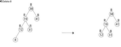


Delete 38
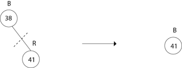
Delete 41
No Tree.
AA TREE
An AA tree in computer science is a form of balanced tree used for storing and retrieving ordered data efficiently. AA trees are named for Arne Andersson, their inventor. AA trees are a variation of the red-black tree, which in turn is an enhancement to the binary search tree. Unlike red-black trees, red nodes on an AA tree can only be added as a right subchild. In other words, no red node can be a left sub-child. This results in the simulation of a 2-3 tree instead of a 2-3-4 tree, which greatly simplifies the maintenance operations. The maintenance algorithms for a red-black tree need to consider seven different shapes to properly balance the tree:

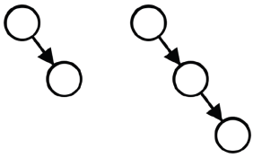
An AA tree on the other hand only needs to consider two shapes due to the strict requirement that only right links can be red:
Balancing Rotations
Typically, AA trees are implemented with levels instead of colors, unlike red-black trees. Each node has a level field, and the following invariants must remain true for the tree to be valid:
Only two operations are needed for maintaining balance in an AA tree. These operations are called skew and split. Skew is a right rotation when an insertion or deletion creates a left horizontal link, which can be thought of as a left red link in the red-black tree context. Split is a conditional left rotation when an insertion or deletion creates two horizontal right links, which once again corresponds to two consecutive red links in red-black trees.
function skew is
input: T, a node representing an AA tree that needs to be rebalanced.
output: Another node representing the rebalanced AA tree.
if nil(T) thenreturn Nilelse if level(left(T)) == level(T) thenSwap the pointers of horizontal left links.
L = left(T)
left(T) := right(L)
right(L) := T return Lelsereturn Tend ifend function
Skew:
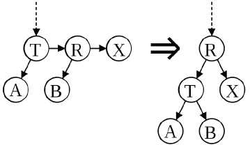
function split is
input: T, a node representing an AA tree that needs to be rebalanced.
output: Another node representing the rebalanced AA tree.
if nil(T) thenreturn Nilelse if level(T) == level(right(right(T))) thenWe have two horizontal right links. Take the middle node,elevate it, and return it.
R = right(T)
right(T) := left(R)
left(R) := T
level(R) := level(R) + 1return Relsereturn Tend ifend function
Split:
Insertion
Insertion begins with the normal binary tree search and insertion procedure. Then, as the call stack unwinds, it's easy to check the validity of the tree and perform any rotations as necessary. If a horizontal left link arises, a skew will be performed, and if two horizontal right links arise, a split will be performed, possibly incrementing the level of the new root node of the current subtree. Note in the code as given above the increment of level(T). This makes necessary to continue checking the validity of the tree as the modifications bubble up from the leaves.
function insert is input: X, the value to be inserted, and T, the root of the tree to insert it into.
output: A balanced version T including X.Do the normal binary tree insertion procedure. Set the result of the recursive call to the correct child in case a new node was createdor the root of the subtree changes.
if nil(T) thenCreate a new leaf node with X.return node(X, 1, Nil, Nil)else if X < value(T) then
left(T) := insert(X, left(T))else if X > value(T) then
right(T) := insert(X, right(T))end if
Note that the case of X == value(T) is unspecified. As given, an insert will have no effect. The implementor may desire differentbehavior. Perform skew and then split. The conditionals that determine whether or not a rotation will occur or not are inside of the procedures, as givenabove.
T := skew(T)
T := split(T)return Tend function
Deletion
As in most balanced binary trees, the deletion of an internal node can be turned into the deletion of a leaf node by swapping the internal node with either its closest predecessor or successor, depending on which are in the tree or the implementor's whims. Retrieving a predecessor is simply a matter of following one left link and then all of the remaining right links. Similarly, the successor can be found by going right once and left until a null pointer is found. Because of the AA property of all nodes of level greater than one having two children, the successor or predecessor node will be in level 1, making their removal trivial.
To re-balance a tree, there are a few approaches. The one described by Andersson in his original paper is the simplest, and it is described here, although actual implementations may opt for a more optimized approach. After a removal, the first step to maintaining tree validity is to lower the level of any nodes whose children are two levels below them, or who are missing children. Then, the entire level must be skewed and split. This approach was favored, because when laid down conceptually, it has three easily understood separate steps:
However, we have to skew and split the entire level this time instead of just a node, complicating our code.
function delete is
input: X, the value to delete, and T, the root of the tree from which it should be deleted.
output: T, balanced, without the value X. if X > value(T) then
right(T) := delete(X, right(T))else if X < value(T) then
left(T) := delete(X, left(T))elseIf we're a leaf, easy, otherwise reduce to leaf case.if leaf(T) then
return Nilelse if nil(left(T)) then
L := successor(T)
right(T) := delete(L, right(T))
value(T) := Lelse
L := predecessor(T)
left(T) := delete(L, left(T))
value(T) := Lend ifend ifRebalance the tree. Decrease the level of all nodes in this levelif
necessary, and then skew and split all nodes in the new level.
T := decrease_level(T)
T := skew(T)
right(T) := skew(right(T))
right(right(T)) := skew(right(right(T)))
T := split(T)
right(T) := split(right(T))
return Tend functionfunction decrease_level is
input: T, a tree for which we want to remove links that skip levels.
output: T with its level decreased.
should_be = min(level(left(T)), level(right(T))) + 1if should_be < level(T) then
level(T) := should_beif should_be < level(right(T)) then
level(right(T)) := should_beend ifend if
return Tend function
A good example of deletion by this algorithm is present in the Andersson paper
Performance
The performance of an AA tree is equivalent to the performance of a red-black tree. While an AA tree makes more rotations than a red-black tree, the simpler algorithms tend to be faster, and all of this balances out to result in similar performance. A red-black tree is more consistent in its performance than an AA tree, but an AA tree tends to be flatter, which results in slightly faster search times.
In computer science, a kd-tree (short for k-dimensional tree) is a space partitioning data structure for organizing points in a k-dimensional space. Kd trees are a useful data structure for several applications, such as searches involving a multidimensional search key (e.g. range searches and nearest neighbor searches). kd-trees are a special case of BSP trees.
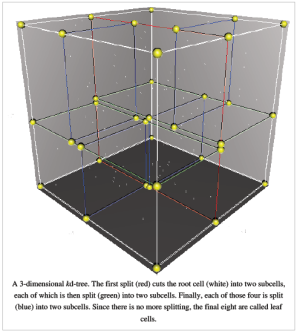
Informal Description
The kd-tree is a binary tree in which every node is a k-dimensional point. Every non-leaf node can be thought of as implicitly generating a splitting hyperplane that divides the space into two parts, known as subspaces. Points to the left of this hyperplane represent the left sub-tree of that node and points right of the hyperplane are represented by the right sub-tree. The hyperplane direction is chosen in the following way: every node in the tree is associated with one of the k-dimensions, with the hyperplane perpendicular to that dimension's axis. So, for example, if for a particular split the "x" axis is chosen, all points in the subtree with a smaller "x" value than the node will appear in the left subtree and all points with larger "x" value will be in the right sub tree. In such a case, the hyperplane would be set by the x-value of the point, and its normal would be the unit x-axis.
Operations on kd-trees
Construction
Since there are many possible ways to choose axis-aligned splitting planes, there are many different ways to construct kd-trees. The canonical method of kd-tree construction has the following constraints:
(Note the assumption that we feed the entire set of points into the algorithm up-front.) This method leads to a balanced kd-tree, in which each leaf node is about the same distance from the root. However, balanced trees are not necessarily optimal for all applications. Note also that it is not required to select the median point. In that case, the result is simply that there is no guarantee that the tree will be balanced. A simple heuristic to avoid coding a complex linear-time median-finding algorithm nor using an O(n log n) sort is to use sort to find the median of a fixed number of randomly selected points to serve as the cut line. Practically this technique often results in nicely balanced trees. Given a list of n points, the following algorithm will construct a balanced kd-tree containing those points.
function kdtree
(list of points pointList, int depth)
{if pointList is emptyreturn nil;else
{// Select axis based on depth so that axis cycles through allvalid valuesvar int axis := depth mod k;
// Sort point list and choose median as pivot elementselect median by axis from pointList;
// Create node and construct subtreesvar tree_node node;
node.location := median;
node.leftChild := kdtree(points in pointList before median,
depth+1);
node.rightChild := kdtree(points in pointList after median,
depth+1);return node;
}
}
##
It is common that points "after" the median include only ones that are greater than or equal to the median. Another approach is to define a "superkey" function that compares the points in other dimensions. Lastly, it may be acceptable to let points equal to the median lie on either side. This algorithm implemented in the Python programming language is as follows:
class Node:passdef kdtree(pointList, depth=0):if not pointList:return# Select axis based on depth so that axis cycles through all valid values
k = len(pointList[0]) # assumes all points have the same dimension
axis = depth % k# Sort point list and choose median as pivot element
pointList.sort(key=lambda point: point[axis])
median = len(pointList)/2 # choose median# Create node and construct subtrees
node = Node()
node.location = pointList[median]
node.leftChild = kdtree(pointList[0:median], depth+1)
node.rightChild = kdtree(pointList[median+1:], depth+1)return node
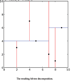
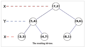
The tree generated is shown on the right. This algorithm creates the invariant that for any node, all the nodes in the left subtree are on one side of a splitting plane, and all the nodes in the right subtree are on the other side. Points that lie on the splitting plane may appear on eithe side. The splitting plane of a node goes through the point associated with that node (referred to in the code as node.location).
The resulting kd-tree decomposition.
Adding elements
One adds a new point to a kd-tree in the same way as one adds an element to any other search tree. First, traverse the tree, starting from the root and moving to either the left or the right child depending on whether the point to be inserted is on the "left" or "right" side of the splitting plane. Once you get to the node under which the child should be located, add the new point as either the left or right child of the leaf node, again depending on which side of the node's splitting plane contains the new node. Adding points in this manner can cause the tree to become unbalanced, leading to decreased tree performance. The rate of tree performance degradation is dependent upon the spatial distribution of tree points being added, and the number of points added in relation to the tree size.
If a tree becomes too unbalanced, it may need to be re-balanced to restore the performance of queries that rely on the tree balancing, such as nearest neighbour searching.
Removing elements
To remove a point from an existing kd-tree, without breaking the invariant, the easiest way is to form the set of all nodes and leaves from the children of the target node, and recreate that part of the tree. This differs from regular search trees in that no child can be selected for a "promotion", since the splitting plane for lower-level nodes is not along the required axis for the current tree level.
Balancing
Balancing a kd-tree requires care. Because kd-trees are sorted in multiple dimensions, the tree rotation technique cannot be used to balance them — this may break the invariant.
Nearest neighbor search
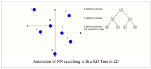
The nearest neighbor (NN) algorithm aims to find the point in the tree which is nearest to a given input point. This search can be done efficiently by using the tree properties to quickly eliminate large portions of the search space. Searching for a nearest neighbor in a kd-tree proceeds as follows:
Animation of NN searching with a KD Tree in 2D
Generally the algorithm uses squared distances for comparison to avoid computing square roots. Additionally, it can save computation by holding the squared current best distance in a variable for comparison.
Sample LUA - NN Searchfunction kdsearchnn( here, point, best )if here == nil thenreturn bestendif best == nil then
best = hereend-- consider the current node --
disthere = distance(here,point)
distbest = distance(best,point)if disthere < distbest then
best = hereend-- search the near branch --
child = child_near(here,point)
best = kdsearchnn( child, point, best )-- search the away branch - maybe --
distbest = distance(best,point)
distaxis = distance_axis(here,point)if distaxis < distbest then
child = child_away(here,point)
best = kdsearchnn( child, point, best )endreturn bestend
Finding the nearest point is an O(log N) operation in the case of randomly distributed points if N. Analyses of binary search trees has found that the worst case search time for an k-dimensional KD tree containing N nodes is given by the following equation .

These poor running times only apply when N is on the order of the number of dimensions. In very high dimensional spaces, the curse of dimensionality causes the algorithm to need to visit many more branches than in lower dimensional spaces. In particular, when the number of points is only slightly higher than the number of dimensions, the algorithm is only slightly better than a linear search of all of the points. The algorithm can be extended in several ways by simple modifications. It can provide the k-Nearest Neighbors to a point by maintaining k current bests instead of just one. Branches are only eliminated when they can't have points closer than any of the k current bests. It can also be converted to an approximation algorithm to run faster.
For example, approximate nearest neighbor searching can be achieved by simply setting an upper bound on the number points to examine in the tree, or by interrupting the search process based upon a real time clock (which may be more appropriate in hardware implementations). Nearest neighbour for points that are in the tree already can be achieved by not updating the refinement for nodes that give zero distance as the result, this has the downside of discarding points that are not unique, but are co-located with the original search point. Approximate nearest neighbor is useful in real time applications such as robotics due to the significant speed increase gained by not searching for the best point exhaustively. One of its implementations is Best Bin First.
High-Dimensional Data
kd-trees are not suitable for efficiently finding the nearest neighbour in high dimensional spaces. As a general rule, if the dimensionality is k, then number of points in the data, N, should be N >> 2k. Otherwise, when kd-trees are used with high -dimensional data, most of the points in the tree will be evaluated and the efficiency is no better than exhaustive search and approximate nearest-neighbour methods are used instead.
Complexity
Variations
Instead of points
Instead of points, a kd-tree can also contain rectangles or hyper rectangles. A 2D rectangle is considered a 4D object (xlow, xhigh, ylow, yhigh). Thus range search becomes the problem of returning all rectangles intersecting the search rectangle. The tree is constructed the usual way with all the rectangles at the leaves. In an orthogonal range search, the opposite coordinate is used when comparing against the median. For example, if the current level is split along xhigh, we check the xlow coordinate of the search rectangle. If the median is less than the xlow coordinate of the search rectangle, then no rectangle in the left branch can ever intersect with the search rectangle and so can be pruned. Otherwise both branches should be traversed. See also interval tree, which is a 1-dimensional special case.
Points only in leaves
It is also possible to define a kd-tree with points stored solely in leaves . This form of kd-tree allows a variety of split mechanics other than the standard median split. The midpoint splitting rule[6] selects on the middle of the longest axis of the space being searched, regardless of the distribution of points. This guarantees that the aspect ratio will be at most 2:1, but the depth is dependent on the distribution of points. A variation, called sliding-midpoint, only splits on the middle if there are points on both sides of the split. Otherwise, it splits on point nearest to the middle. Maneewongvatana and Mount show that this offers "good enough" performance on common data sets. Using sliding-midpoint, an approximate nearest neighbor query can be answered in Approximate range counting can be answered in

with this method.
A splay tree is a self-balancing binary search tree with the additional property that recently accessed elements are quick to access again. It performs basic operations such as insertion, look-up and removal in O(log(n)) amortized time. For many non-uniform sequences of operations, splay trees perform better than other search trees, even when the specific pattern of the sequence is unknown. The splay tree was invented by Daniel Dominic Sleator and Robert Endre Tarjan in 1985.
All normal operations on a binary search tree are combined with one basic operation, called splaying. Splaying the tree for a certain element rearranges the tree so that the element is placed at the root of the tree. One way to do this is to first perform a standard binary tree search for the element in question, and then use tree rotations in a specific fashion to bring the element to the top. Alternatively, a top-down algorithm can combine the search and the tree reorganization into a single phase.
Advantages
Good performance for a splay tree depends on the fact that it is self -balancing, and indeed self-optimizing, in that frequently accessed nodes will move nearer to the root where they can be accessed more quickly. This is an advantage for nearly all practical applications, and is particularly useful for implementing caches and garbage collection algorithms.
Advantages include:
Disadvantages
Disadvantages:
One worst-case issue with the basic splay tree algorithm is that of sequentially accessing all the elements of the tree in the sorted order. This leaves the tree completely unbalanced (this takes n accesses, each an O(log n) operation). Reaccessing the first item triggers an operation that takes O(n) Operations to rebalance the tree before returning the first item. This is a significant delay for that final operation, although the amortized performance over the entire sequence is actually O(log n). However, recent research shows that randomly rebalancing the tree can avoid this unbalancing effect and give similar performance to the other self-balancing algorithms.
Splaying
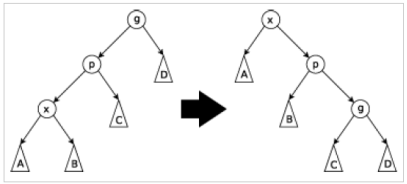
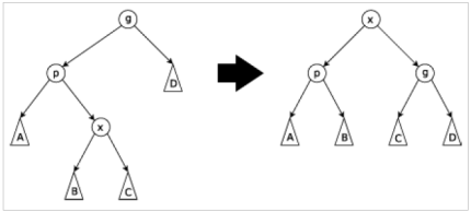
When a node x is accessed, a splay operation is performed on x to move it to the root. To perform a splay operation we carry out a sequence of splay steps, each of which moves x closer to the root. By performing a splay operation on the node of interest after every access, the recently accessed nodes are kept near the root and the tree remains roughly balanced, so that we achieve the desired amortized time bounds. Each particular step depends on three factors:
The three types of splay steps are:
Zig Step: This step is done when p is the root. The tree is rotated on the edge between x and p. Zig steps exist to deal with the parity issue and will be done only as the last step in a splay operation and only when x has odd depth at the beginning of the operation.
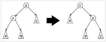
Zig-zag Step: This step is done when p is not the root and x is a right child and p is a left child or vice versa. The tree is rotated on the edge between x and p, then rotated on the edge between x and its new parent g.
Insertion
To insert a node x into a splay tree, we first insert it as with a normal binary search tree. Then we splay the new node x to the top of the tree.
Deletion
To delete a node x, we use the same method as with a binary search tree. If x has two children, we replace its value with either the rightmost node of its left subtree (its in-order predecessor) or the leftmost node of its right subtree (its in-order successor). Then we remove that node instead. In this way, deletion is reduced to the problem of removing a node with 0 or 1 children. After deletion, we splay the parent of the removed node to the top of the tree.
Code in "C" language
A complete program of splay tree written in C is uploaded at this location
Splay operation in BST
Here x is the node on which the splay operation is performed and root is the root node of the tree.
void splay (struct node *x, struct node *root)
{
node *p,*g;
/*check if node x is the root node*/
if(x==root);
/*Performs Zig step*/
else if(x->parent==root)
{
if(x==(x->parent)->left)
rightrotation(root);
else
leftrotation(root);
}
else
{
p=x->parent; /*now points to parent of x*/
g=p->parent; /*now points to parent of x's parent*/
/*Performs the Zig-zig step when x is left and x's parent is left*/
if(x==p->left&&p==g->left)
{
rightrotation(g);
rightrotation(p);
}
/*Performs the Zig-zig step when x is right and x's parent is right*/
else if(x==p->right&&p==g->right)
{
leftrotation(g);
leftrotation(p);
}
/*Performs the Zig-zag step when x's is right and x's parent is left*/
else if(x==p->right&&p==g->left)
{
leftrotation(p);
rightrotation(g);
}
/*Performs the Zig-zag step when x's is left and x's parent is right*/
else if(x==p->left&&p==g->right)
{
rightrotation(p);
leftrotation(g);
}
splay(x, root);
}
}
Analysis
A simple amortized analysis of static splay trees can be carried out using the potential method. Suppose that size(r) is the number of nodes in the subtree rooted at r (including r) and rank(r) = log2(size(r)). Then the potential function P(t) for a splay tree t is the sum of the ranks of all the nodes in the tree. This will tend to be high for poorly-balanced trees, and low for well-balanced trees. We can bound the amortized cost of any zig-zig or zig-zag operation by:
amortized cost = cost + P(tf) - P(ti) ≤ 3(rankf(x) - ranki(x)),
where x is the node being moved towards the root, and the subscripts "f" and "i" indicate after and before the operation, respectively. When summed over the entire splay operation, this telescopes to 3(rank(root)) which is O(log n). Since there's at most one zig operation, this only adds a constant.
Performance theorems
There are several theorems and conjectures regarding the worst-case runtime for performing a sequence S of m accesses in a splay tree containing n elements.
Balance Theorem
The cost of performing the sequence S is 0(m(1+log n)+n log n)In other words, splay trees perform as well as static balanced binary search trees on sequences of at least n accesses.
Static Optimality Theorem
Let qi be the number of times element i is accessed in S. The cost of performing S is

In other words, splay trees perform as well as optimum static binary search trees on sequences of at least n accesses.
Static Finger Theorem
Let be the element accessed in the jthaccess of S and let f be any fixed element (the finger). The cost of performing S is

Working Set Theorem
Let t(j) be the number of distinct elements accessed between access j and the previous time element was accessed. The cost of performing S is

Dynamic Finger Theorem
The cost of performing S is

Scanning Theorem
Also known as the Sequential Access Theorem. Accessing the n elements of a splay tree in symmetric order takes O(n) time, regardless of the initial structure of the splay tree. The tightest upper bound proven so far is 4.5n.
Dynamic optimality conjecture
In addition to the proven performance guarantees for splay trees there is an unproven conjecture of great interest from the original Sleator and Tarjan paper. This conjecture is known as the dynamic optimality conjecture and it basically claims that splay trees perform as well as any other binary search tree algorithm up to a constant factor.
Dynamic Optimality Conjecture: Let A be any binary search tree algorithm that accesses an element by traversing the path from the root to at a cost of d(x)+1 and that between accesses can make any rotations in the tree at a cost of 1 per rotation. Let A(S) be the cost for to perform the sequence of accesses. Then the cost for a splay tree to perform the same accesses is 0(n+A(s)).
There are several corollaries of the dynamic optimality conjecture that remain unproven:
Traversal Conjecture:[1] Let T1 and T2 be two splay trees containing the same elements. Let be the sequence obtained by visiting the elements in T2 in preorder (i.e. depth first search order). The total cost of performing the sequence of accesses on T1 is is O(n)
Deque Conjecture: Let be a sequence of M double-ended queue operations (push, pop, inject, eject). Then the cost of performing on a splay tree is o(m+n)
Split Conjecture:Let be any permutation of the elements of the splay tree. Then the cost of deleting the elements in the order is O(n)
Key takeaway
AVL Tree is invented by GM Adelson - Velsky and EM Landis in 1962. The tree is named AVL in honour of its inventors.
AVL Tree can be defined as height balanced binary search tree in which each node is associated with a balance factor which is calculated by subtracting the height of its right sub-tree from that of its left sub-tree.
Tree is said to be balanced if balance factor of each node is in between -1 to 1, otherwise, the tree will be unbalanced and need to be balanced.
References:
1. Horowitz, Sahani, Dinesh Mehata, ―Fundamentals of Data Structures in C++‖, Galgotia Publisher, ISBN: 8175152788, 9788175152786.
2. M Folk, B Zoellick, G. Riccardi, ―File Structures‖, Pearson Education, ISBN:81-7758-37-5
3. Peter Brass, ―Advanced Data Structures‖, Cambridge University Press, ISBN: 978-1-107- 43982-5
4. A. Aho, J. Hopcroft, J. Ulman, ―Data Structures and Algorithms‖, Pearson Education, 1998, ISBN-0-201-43578-0.
5. Michael J Folk, ―File Structures an Object-Oriented Approach with C++‖, Pearson Education, ISBN: 81-7758-373-5.
6. Sartaj Sahani, ―Data Structures, Algorithms and Applications in C++‖, Second Edition, University Press, ISBN:81-7371522 X.
7. G A V Pai, ―Data Structures and Algorithms‖, The McGraw-Hill Companies, ISBN - 9780070667266.
8. Goodrich, Tamassia, Goldwasser, ―Data Structures and Algorithms in Java‖, Wiley Publication, ISBN: 9788126551903

