Unit-3
Statistics
Professor Bowley defines the average as-
“Statistical constants which enable us to comprehend in a single effort the significance of the whole”
An average is a single value that is the best representative for a given data set.
Measures of central tendency show the tendency of some central values around which data tend to cluster.
The following are the various measures of central tendency-
1. Arithmetic mean
2. Median
3. Mode
4. Weighted mean
5. Geometric mean
6. Harmonic mean
The arithmetic mean or mean-
The arithmetic mean is a value which is the sum of all observation divided by a total number of observations of the given data set.
If there are n numbers in a dataset-  then the arithmetic mean will be-

If the numbers along with frequencies are given then mean can be defined as-

Example-1: Find the mean of 26, 15, 29, 36, 35, 30, 14, 21, 25 .
Sol.


Example-2: Find the mean of the following dataset.
x | 20 | 30 | 40 |
f | 5 | 6 | 4 |
Sol.
We have the following table-
X | F | Fx |
20 | 5 | 100 |
30 | 6 | 180 |
40 | 7 | 160 |
| Sum = 15 | Sum = 440 |
Then Mean will be-


Short cut method
Let a be the assumed mean, d the deviation of the variate x from a. Then

Example1. Find the arithmetic mean for the following distribution:
Class | 0-10 | 10-20 | 20-30 | 30-40 | 40-50 |
Frequency | 7 | 8 | 20 | 10 | 5 |
Solution. Let assumed mean (a) = 25
Class | Mid value
| Frequency |
|
|
40— 50 |
|
|
|
|
Total |
|
|
|
|

(c) Step deviation method
Let  be the assumed mean,
  the width of the class interval and

Example 2. Find the arithmetic mean of the data given in example by step deviation method
Solution. Let 
Class | Mid‐value
| frequency
|
|
|
|
|
|
|
|
Total |
|
|
|
|

Median-
Median is the mid-value of the given data when it is arranged in ascending or descending order.
1. If the total number of values in the data set is odd then the median is the value of  item.
item.
Note-The data should be arranged in ascending r descending order
2. If the total number of values in the data set is even then the median is the mean of the  item.
item.
Example: Find the median of the data given below-
7, 8, 9, 3, 4, 10
Sol.
Arrange the data in ascending order-
3, 4, 7, 8, 9, 10
So there total 6 (even) observations, then-


=
Median for grouped data-

Here,


Example: Find the median of the following dataset-

Sol.
Class interval | Frequency | Cumulative frequency |
0 - 10 | 3 | 3 |
10 – 20 | 5 | 8 |
20 – 30 | 7 | 15 |
30 – 40 | 9 | 24 |
40 – 50 | 4 | 28 |

So that median class is 20-30.
Now putting the values in the formula-


So that the median is 28.57
Example: Find the value of Median from the following data:
No. of days for which absent (less than) |
|
|
|
|
|
|
|
|
|
No. of students |
|
|
|
|
|
|
|
|
|
Solution. The given cumulative frequency distribution will first be converted into ordinary frequency as under
Class Interval | Cumulative frequency | Ordinary frequency |
0-5 5-10
15-20 20-25 25-35 30-35 35-40 40-45 | 29
465 582 634 644 650 653 655 | 29=29 224-29=195 465-224= 582-465=117 634-582=52 644-634=10 650-644=6 653-650=3 655-653=2 |
Median  size of
 or 327.
 Item
Item
327.  Item lies in 10‐15 which is the median class.

Where  stands for the lower limit of the median class,
 stands for the total frequency,
 stands for the cumulative frequency just preceding the median class,
  stands for class interval
 stands for frequency for the median class.
Median 

Mode-
A value in the data which is most frequent is known as mode.
Example: Find the mode of the following data points-

Sol. Here 6 has the highest frequency so that the mode is 6.
Mode for grouped data-

Here,


Example: Find the mode of the following dataset-

Sol.
Class interval | Frequency |
0 - 10 | 3 |
10 – 20 | 5 |
20 – 30 | 7 |
30 – 40 | 9 |
40 – 50 | 4 |
Here the highest frequency is 9. So that the modal class is 40-50,
Put the values in the given data-


Hence the mode is 42.86
Example: Find the mode from the following data:
Age | 0-6 | 6-12 | 12-18 | 18-24 | 24-30 | 30-36 | 36-42 |
Frequency | 6 | 11 | 25 | 35 | 18 | 12 | 6 |
Solution.
Age | Frequency | Cumulative frequency |
0-6 6-12 12-18
24-30 30-36 36-42 | 6 11 25 35
12 6 | 6 17 42 77 95 107 113 |
Mode


GEOMETRIC MEAN
 , ,
, , be
be  values of variates
  , then the geometric mean

Example 7. Find the geometric mean of 4, 8, 16.
Solution. .
.
HARMONIC MEAN
The harmonic mean of a series of values is defined as the reciprocal of the arithmetic mean of their reciprocals. Thus  be the harmonic mean, then

Example 8:Calculate the harmonic mean of 4, 8, 16.
Solution:


Note-
1. 
2. 
3. Mean – Mode = [Mean - Median]
According to Spiegel-
“The degree to which numerical data tend to spread about an average value is called the variation or dispersion of data”
The different measures of dispersion are-
1. Range
2. Quartile deviation
3. Mean deviation
4. Standard deviation
5. Variance
Range-
This is one of the simplest measures of dispersion. The difference between the maximum and minimum value of the dataset is known as the range.
Range = Max. value – Min. value
Example- Find the range of the data- 8, 5, 6, 4, 7, 10, 12, 15, 25, 30
Sol. Here the maximum value is 30 and the minimum value is 4 so that the range is-
30 – 4 = 26
Coefficient of range-
The coefficient of range can be calculated as follows-
Coefficient of Range = 
Quartile deviation-


Example- Find the quartile deviation of the following data-
Class interval | 0-10 | 10-20 | 20-30 | 30-40 | 40-50 |
Frequency | 3 | 5 | 7 | 9 | 4 |
Sol.
Here N/4 = 28/4 = 7 so that the 7’th observation falls in class 10 – 20.
And
3N/4 = 21, and 21’st observation falls in the interval 30 – 40 which is the third quartile.
The quartiles can be calculated as below-

And

Hence the quartile deviation is-

Mean deviation-
The mean deviation can be defined as-

Here A is assumed mean.


Example: Find the mean deviation from the mean of the following data-
Class interval | 0-6 | 6-12 | 12-18 | 18-24 | 24-30 |
Frequency | 8 | 10 | 12 | 9 | 5 |
Sol.
Class interval | Mid-value | Frequency | d = x - a | f.d | |x - 14| | f |x - 14| |
0-6 | 3 | 8 | -12 | -96 | 11 | 88 |
6-12 | 9 | 10 | -6 | -60 | 5 | 50 |
12-18 | 15 | 12 | 0 | 0 | 1 | 12 |
18-24 | 21 | 9 | 6 | 54 | 7 | 63 |
24-30 | 27 | 5 | 12 | 60 | 13 | 65 |
Total |
| 44 |
| -42 |
| 278 |

Then mean deviation from mean-

Standard deviation:
It is defined as the positive square root of the arithmetic mean of the square of the deviation of the given values from their arithmetic mean. It is denoted by the symbol  .
.

Where  is A.M of the distribution
  . We have more formulae to calculate the standard deviation.

In frequency distribution from, we put  where H is generally taken as width of class interval
Shortcut formula to calculate standard deviation-

The square of the standard deviation is called known as a variance.

Example-1: Compute the variance and standard deviation.
Class | Frequency |
0-10 | 3 |
10-20 | 5 |
20-30 | 7 |
30-40 | 9 |
40-50 | 4 |
Sol.
Class | Mid-value (x) | Frequency (f) |
|
0-10 | 5 | 3 | 1470.924 |
10-20 | 15 | 5 | 737.250 |
20-30 | 25 | 7 | 32.1441 |
30-40 | 35 | 9 | 555.606 |
40-50 | 45 | 4 | 1275.504 |
Sum |
|
| 4071.428 |

Then standard deviation,

Example-2: Calculate the standard deviation of the following frequency distribution-
Weight | 60 – 62 | 63 – 65 | 66 – 68 | 69 – 71 | 72 – 74 |
item | 5 | 18 | 42 | 27 | 8 |
Sol.
Weight | Item (f) | X | d = x – 67 | f.d |
|
60 – 62 | 5 | 61 | -6 | -30 | 180 |
63 – 65 | 18 | 64 | -3 | -54 | 162 |
66 – 68 | 42 | 67 | 0 | 0 | 0 |
69 – 71 | 27 | 70 | 3 | 81 | 243 |
72 – 74 | 8 | 73 | 6 | 48 | 288 |
Total |
100 |
|
|
45 |
873 |


Example: Calculate S.D for the following distribution.
Solution:
Coefficient of variation can be calculated as-

Note- The lower value of C.V, the more constancy of data
Example- If student A has a mean 50 with SD 10. Another student B has a mean of 30 with SD = 3.
Which one is the best performer?
Sol. We calculate C.V.-


And

Here B has a lower C.V. so that student B is the best performer.
Example: Calculate coefficient variation for the following frequency distribution.


The rth moment of a variable x about the mean x is usually denoted by is given by

The rth moment of a variable x about any point a is defined by


The relation between moments about mean and moment about any point:

 where
where and
and 


In particular


Note. 1. The sum of the coefficients of the various terms on the right‐hand side is zero.
2. The dimension of each term on the right‐hand side is the same as that of terms on the left.
MOMENT GENERATING FUNCTION
The moment generating function of the variate  about
about  is defined as the expected value of
  and is denoted by
  .
.


where  , ‘ is the moment of order
  about
about 
Hence  coefficient of
  or
or 
again  )
) 
Thus, the moment generating function about the point  moment generating function about the origin.
Skewness-
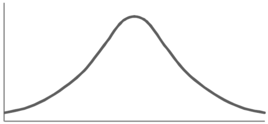
The word skewness means lack of symmetry-
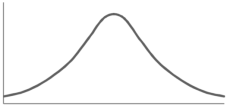
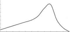
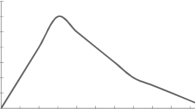
The examples of the symmetric curve, positively skewed, and negatively skewed curves are given as follows-
1. Symmetric curve-
2. Positively skewed-
3. Negatively skewed-
To measure the skewness we use Karl Pearson’s coefficient of skewness.
Then the formula is as follows-

Note- the value of Karl Pearson’s coefficient of skewness lies between -1 to +1.
Kurtosis-
It is the measurement of the degree of peakedness of a distribution
Kurtosis is measured as-
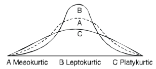
Calculation of kurtosis-
The second and fourth central moments are used to measure kurtosis.
We use Karl Pearson’s formula to calculate kurtosis-

Now, three conditions arise-
1. If  , then the curve is mesokurtic.
2. If  , then the curve is platykurtic
3. if  , then the curve is said to be leptokurtic.
Example: If the coefficient of skewness is 0.64. The standard deviation is 13 and the mean is 59.2, then find the mode and median.
Sol.
We know that-

So that-


And we also know that-


Example: Calculate Karl Pearson’s coefficient of skewness of marks obtained by 150 students.

Sol. The mode is not well defined so that first we calculate mean and median-
Class | f | x | CF |
| fd |
|
0-10 | 10 | 5 | 10 | -3 | -30 | 90 |
10-20 | 40 | 15 | 50 | -2 | -80 | 160 |
20-30 | 20 | 25 | 70 | -1 | -20 | 20 |
30-40 | 0 | 35 | 70 | 0 | 0 | 0 |
40-50 | 10 | 45 | 80 | 1 | 10 | 10 |
50-60 | 40 | 55 | 120 | 2 | 80 | 160 |
60-70 | 16 | 65 | 136 | 3 | 48 | 144 |
70-80 | 14 | 75 | 150 | 4 | 56 | 244 |
Now,


And

Standard deviation-

Then-


Method of Least Squares:
Let  … (1)
… (1)
be the straight line to be fitted to the given data points  .
.
Let  be the theoretical value for
  .
.
Then 


For S to be minimum
 or
or
[To generalize  ,
,  is written as y]
 or
or
On Simplification equation (2) and (3) becomes


The equations (3) and (4) are known as Normal equations.
On solving equations (3) and (4), we get the values of a and b.
(b) To fit the parabola:

The normal equations are


On solving three equations, we get the values of a, b and c.
Note:
1. The normal equation (4) has been obtained by putting on both sides of
equation (1). Equation (5) is obtained by multiplying  on both sides of (1).
2. The normal equation (7), (8), (9) are obtained by multiply by
 and
and on both sides of equation (6).
Example: Find the best values of a and b so that  fit the data given in the table.
X | 0 | 1 | 2 | 3 | 4 |
Y | 1 | 2.9 | 4.8 | 6.7 | 8.6 |
Solution: 
|
|
|
|
0 | 1 | 0 | 0 |
1 | 2.9 | 2.9 | 1 |
2 | 4.8 | 9.6 | 4 |
3 | 6.7 | 20.1 | 9 |
4 | 8.6 | 13.4 | 16 |
| |
|
|
Normal equations  …. (2)
 …. (3)
On putting the values of  in (2) and (3), we have
 …. (4)
 …. (5)
On solving (4) and (5), we get

On Substituting the values of a and b in (1), we get

Example: By the method of least squats, find the straight line that best fits the following data:
| 1 | 2 | 3 | 4 | 5 |
| 14 | 27 | 40 | 55 | 68 |
Solution: Let the equation of the straight line best fit be  …. (1)
|
|
|
|
1 | 14 | 14 | 1 |
2 | 27 | 54 | 4 |
3 | 40 | 120 | 9 |
4 | 55 | 220 | 16 |
5 | 68 | 340 | 25 |
|
|
|
|
Normal equations are

Putting the values of  in (2) and (3), we have

On solving (4) and (5), we get

On Substituting the values of a and b in (1), we get

Example: Find the least-squares approximation of the second degree for the discrete data.
| -2 | -1 | 0 | 1 | 2 |
| 15 | 1 | 1 | 3 | 19 |
Solution:
Let the equation of second-degree polynomial be 
|
|
|
|
|
|
|
-2 | 15 | -30 | 4 | 60 | -8 | 16 |
-1 | 1 | -1 | 1 | 1 | -1 | 1 |
0 | 1 | 0 | 0 | 0 | 0 | 0 |
1 | 3 | 3 | 1 | 3 | 1 | 1 |
2 | 19 | 38 | 4 | 76 | 8 | 16 |
|
|
|
|
|
|
|
Normal equations are

On putting the values of  in equations (2), (3), (4), we have

On solving (5), (6), (7), we get 
The required polynomial of the second degree is 
Change of Scale: If the data is of equal interval in large numbers then we change the scale as  .
.
Example: Fit a second-degree parabola to the following data by the least-squares method.
| 1929 | 1930 | 1931 | 1932 | 1933 | 1934 | 1935 | 1936 | 1937 |
| 352 | 356 | 357 | 358 | 360 | 361 | 361 | 360 | 359 |
Solution: Taking 
Taking 

The equation  is transformed into
|
|
|
|
|
|
|
|
|
1929 | -4 | 352 | -5 | 20 | 16 | -80 | -64 | 256 |
1930 | -3 | 360 | -1 | 3 | 9 | -9 | -27 | 81 |
1931 | -2 | 357 | 0 | 0 | 4 | 0 | -8 | 16 |
1932 | -1 | 358 | 1 | -1 | 1 | 1 | -1 | 1 |
1933 | 0 | 360 | 3 | 0 | 0 | 0 | 0 | 0 |
1934 | 1 | 361 | 4 | 4 | 1 | 4 | 1 | 1 |
1935 | 2 | 361 | 4 | 8 | 4 | 16 | 8 | 16 |
1936 | 3 | 360 | 3 | 9 | 9 | 27 | 27 | 81 |
1937 | 4 | 359 | 2 | 8 | 16 | 32 | 64 | 256 |
Total |
|
|
|
|
|
|
|
|
Normal equations are


On solving these equations, we get 


Example: Fit a second-degree parabola to the following data:
x | 0 | 1 | 2 | 3 | 4 |
y | 1 | 1.8 | 1.3 | 2.5 | 6.3 |
Solution: Let  and
and  so that the parabola of fit
  becomes
 …. (i)
The normal equations are


Saving these as simultaneous equations we get

(i) becomes

Or 
Hence 
Example: Fit a second degree parabola to the following data:
| 1.5 | 2 | 2.5 | 3 | 3.5 | 4 |
| 1.3 | 1.6 | 2 | 2.7 | 3.4 | 4.1 |
Solution: We shift the origin to (2.5, 0) and take 0.5 as the new unit. This amounts to changing the variable  to X, by the relation
Let the parabola of fit be  . The values of
  etc., ae calculated below:
|
|
|
|
|
|
|
|
1.0 | -3 | 1.1 | -3.3 | 9 | 9.9 | -27 | 81 |
1.5 | -2 | 1.3 | -2.6 | 4 | 5.2 | -8 | 16 |
2.0 | -1 | 1.6 | -1.6 | 1 | 1.6 | -1 | 1 |
2.5 | 0 | 2 | 0 | 0 | 0 | 0 | 0 |
3.0 | 1 | 2.7 | 2.7 | 1 | 2.7 | 1 | 1 |
3.5 | 2 | 3.4 | 6.8 | 4 | 13.6 | 8 | 16 |
4.0 | 3 | 4.1 | 12.3 | 9 | 36.9 | 27 | 81 |
Total | 0 | 16.2 | 14.2 | 28 | 69.9 | 0 | 196 |
The normal equations are

Solving these as simultaneous equations, we get


Replacing X by  in the above equation, we get

Which simplifies by  . This is the required parabola of best fit.
When two variables are related in such a way that a change in the value of one variable affects the value of the other variable, then these two variables are said to be correlated and there is a correlation between two variables.
Example- Height and weight of the persons of a group.
The correlation is said to be a perfect correlation if two variables vary in such a way that their ratio is constant always.
Scatter diagram-
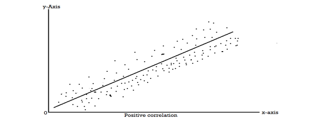
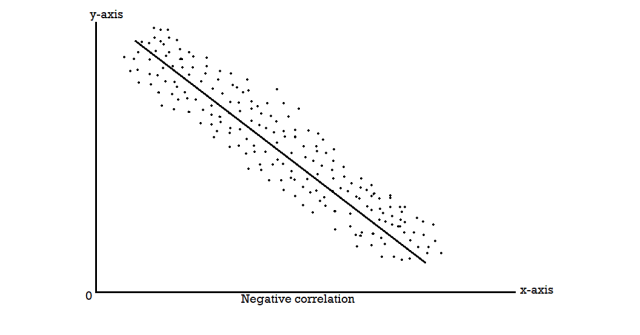
Karl Pearson’s coefficient of correlation-

Here-  and
and 

Note-
1. Correlation coefficient always lies between -1 and +1.
2. Correlation coefficient is independent of the change of origin and scale.
3. If the two variables are independent then the correlation coefficient between them is zero.
Correlation coefficient | Type of correlation |
+1 | Perfect positive correlation |
-1 | Perfect negative correlation |
0.25 | Weak positive correlation |
0.75 | Strong positive correlation |
-0.25 | Weak negative correlation |
-0.75 | Strong negative correlation |
0 | No correlation |
Example: Find the correlation coefficient between age and weight of the following data-
Age | 30 | 44 | 45 | 43 | 34 | 44 |
Weight | 56 | 55 | 60 | 64 | 62 | 63 |
Sol.
x | y |
|
|
|
| ( |
30 | 56 | -10 | 100 | -4 | 16 | 40 |
44 | 55 | 4 | 16 | -5 | 25 | -20 |
45 | 60 | 5 | 25 | 0 | 0 | 0 |
43 | 64 | 3 | 9 | 4 | 16 | 12 |
34 | 62 | -6 | 36 | 2 | 4 | -12 |
44 | 63 | 4 | 16 | 3 | 9 | 12 |
Sum= 240 |
360 |
0 |
202 |
0 |
70
|
32 |
Karl Pearson’s coefficient of correlation-

Here the correlation coefficient is 0.27. which is the positive correlation (weak positive correlation), this indicates that as age increases, the weight also increases.
Short-cut method to calculate correlation coefficient-

Here,


Example: Find the correlation coefficient between the values X and Y of the dataset given below by using the short-cut method-
X | 10 | 20 | 30 | 40 | 50 |
Y | 90 | 85 | 80 | 60 | 45 |
Sol.
X | Y |
|
|
|
|
|
10 | 90 | -20 | 400 | 20 | 400 | -400 |
20 | 85 | -10 | 100 | 15 | 225 | -150 |
30 | 80 | 0 | 0 | 10 | 100 | 0 |
40 | 60 | 10 | 100 | -10 | 100 | -100 |
50 | 45 | 20 | 400 | -25 | 625 | -500 |
Sum = 150 |
360 |
0 |
1000 |
10 |
1450 |
-1150 |
Short-cut method to calculate correlation coefficient-


Spearman’s rank correlation-
When the ranks are given instead of the scores, then we use Spearman’s rank correlation to find out the correlation between the variables.
Spearman’s rank correlation coefficient can be defined as-

Example: Compute the Spearman’s rank correlation coefficient of the dataset given below-
Person | A | B | C | D | E | F | G | H | I | J |
Rank in test-1 | 9 | 10 | 6 | 5 | 7 | 2 | 4 | 8 | 1 | 3 |
Rank in test-2 | 1 | 2 | 3 | 4 | 5 | 6 | 7 | 8 | 9 | 10 |
Sol.
Person | Rank in test-1 | Rank in test-2 | d = |
|
A | 9 | 1 | 8 | 64 |
B | 10 | 2 | 8 | 64 |
C | 6 | 3 | 3 | 9 |
D | 5 | 4 | 1 | 1 |
E | 7 | 5 | 2 | 4 |
F | 2 | 6 | -4 | 16 |
G | 4 | 7 | -3 | 9 |
H | 8 | 8 | 0 | 0 |
I | 1 | 9 | -8 | 64 |
J | 3 | 10 | -7 | 49 |
Sum |
|
|
| 280 |


Regression-
Regression is the measure of the average relationship between the independent and dependent variable
Regression can be used for two or more than two variables.
There are two types of variables in regression analysis.
1. Independent variable
2. Dependent variable
The variable which is used for prediction is called the independent variable.
It is known as a predictor or regressor.
The variable whose value is predicted by an independent variable is called the dependent variable or regressed or explained variable.
The scatter diagram shows the relationship between the independent and dependent variable, then the scatter diagram will be more or less concentrated around a curve, which is called the curve of regression.
When we find the curve as a straight line then it is known as the line of regression and the regression is called linear regression.
Note- regression line is the best fit line that expresses the average relation between variables.
Equation of the line of regression-
Let
y = a + bx ………….. (1)
is the equation of the line of y on x.
Let  be the estimated value of
  for the given value of
  .
.
So that, According to the principle of least squares, we have the determined ‘a’ and ‘b’ so that the sum of squares of deviations of observed values of y from expected values of y,
That means-

Or
 …….. (2)
Is the minimum.
Form the concept of maxima and minima, we partially differentiate U with respect to ‘a’ and ‘b’ and equate to zero.
Which means


And


These equations (3) and (4) are known as the normal equation for a straight line.
Now divide equation (3) by n, we get-

This indicates that the regression line of y on x passes through the point .
.
We know that-

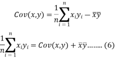
The variance of variable x can be expressed as-


Dividing equation (4) by n, we get-

From equation (6), (7), and (8)-

Multiply (5) by , we get-

Subtracting equation (10) from equation (9), we get-


Since ‘b’ is the slope of the line of regression y on x and the line of regression passes through the point ( ), so that the equation of the line of regression of y on x is-


This is known as the regression line of y on x.
Note-
 are the coefficients of regression.
2. 
Example: Two variables X and Y are given in the dataset below, find the two lines of regression.
x | 65 | 66 | 67 | 67 | 68 | 69 | 70 | 71 |
y | 66 | 68 | 65 | 69 | 74 | 73 | 72 | 70 |
Sol.
The two lines of regression can be expressed as-

And

x | y |
|
| xy |
65 | 66 | 4225 | 4356 | 4290 |
66 | 68 | 4356 | 4624 | 4488 |
67 | 65 | 4489 | 4225 | 4355 |
67 | 69 | 4489 | 4761 | 4623 |
68 | 74 | 4624 | 5476 | 5032 |
69 | 73 | 4761 | 5329 | 5037 |
70 | 72 | 4900 | 5184 | 5040 |
71 | 70 | 5041 | 4900 | 4970 |
Sum = 543 | 557 | 36885 | 38855 | 37835 |
Now-

And

The standard deviation of x-


Similarly-


Correlation coefficient-


Put these values in the regression line equation, we get
Regression line y on x-


Regression line x on y-


A regression line can also be found by the following method-
Example: Find the regression line of y on x for the given dataset.
X | 4.3 | 4.5 | 5.9 | 5.6 | 6.1 | 5.2 | 3.8 | 2.1 |
Y | 12.6 | 12.1 | 11.6 | 11.8 | 11.4 | 11.8 | 13.2 | 14.1 |
Sol.
Let y = a + bx is the line of regression of y on x, where ‘a’ and ‘b’ are given as-


We will make the following table-
x | y | Xy |
|
4.3 | 12.6 | 54.18 | 18.49 |
4.5 | 12.1 | 54.45 | 20.25 |
5.9 | 11.6 | 68.44 | 34.81 |
5.6 | 11.8 | 66.08 | 31.36 |
6.1 | 11.4 | 69.54 | 37.21 |
5.2 | 11.8 | 61.36 | 27.04 |
3.8 | 13.2 | 50.16 | 14.44 |
2.1 | 14.1 | 29.61 | 4.41 |
Sum = 37.5 | 98.6 | 453.82 | 188.01 |
Using the above equations we get-


On solving these both equations, we get-
a = 15.49 and b = -0.675
So that the regression line is –
y = 15.49 – 0.675x
Note – Standard error of predictions can be found by the formula given below-
Difference between regression and correlation-
1. Correlation is the linear relationship between two variables while regression is the average relationship between two or more variables.
2. There are only limited applications of correlation as it gives the strength of linear relationship while the regression is to predict the value of the dependent variable for the given values of independent variables.
3. Correlation does not consider dependent and independent variables while regression considers one dependent variable and other independent variables.
Besides, to study the reliability of regression estimates we require to know the standard error.
The standard error of regression estimate of y on  is
is
The Standard error of Regression estimate of  on
on  is
is
1. Discuss the Reliability of Regression Estimates:
The standard error of Regression of estimates of y on x is
 …..(Standard error of Regression of estimates of y on x is )
References
1. Erwin Kreyszig, Advanced Engineering Mathematics, 9thEdition, John Wiley & Sons, 2006.
2. N.P. Bali and Manish Goyal, A textbook of Engineering Mathematics, Laxmi Publications.
3. Higher engineering mathematic, Dr. B.S. Grewal, Khanna publishers


