Unit - 2
Statistical Inference
The way information is processed as created insights supplement decision-making is the most important part of Data Science. Statistics serves as a foundation for solving various organisational difficulties because dealing with business challenges necessitates anticipating the occurrence of events. When Data Scientists employ Statistics for Data Analytics, they can create complicated models that can provide Big Data insights and help businesses optimise their operations more effectively. Although statistics has long been used in business decisions, the exponential growth of data, processing, and advances in Data Science have resulted in the proliferation of statistics with Big Data.
This article gives you a thorough introduction of statistics' role in data analytics and data science. It also goes through the many types of statistics and key principles, which will help you understand how to apply statistics in the Data Science and Analytics domain.
Benefits
The following are some of the advantages of using statistics for Data Analytics and Data Science:
● Statistics aids in the gathering of information about business activities, making it a crucial component of any Data Science and Analytics project's life cycle.
● It is important in data preparation and feature engineering, in addition to comprehending statistical measures.
● It aids in the visualisation of statistics in order to comprehend patterns and trends in quantitative data.
Application of Statistics for Data Analytics and Data Science
Statistics are no longer expected to be used for computing a quantity measure; they are now required in every business domain for sophisticated analytics. The following are the most essential statistics applications for data analytics and data science:
● Building Machine Learning Algorithms: The connection between statistics and data science and analytics has provided as a foundation for various machine learning algorithms such as logistic regression, naive Bayes, and many more that have evolved with the importance of statistical summary in mind.
● Business Intelligence: Statistics is frequently used in the industry for business processes, since we arrive at a decisive word with a level of certainty. This level of certainty is used to make forecasts and foresee likely outcomes for plans to be implemented.
Statistics are crucial for comprehending the behaviour of a set of attributes and the relationships they share. Data Science and Analytics also necessitate significant math and programming skills, thus statistics is the first step toward comprehending the Data Science and Analytics process. The findings obtained via the use of Statistics for Data Analytics have aided in the generation of insights from data that drive business growth in the industry, allowing the company to stay ahead of the competition.
You must move data from diverse sources into a common Data Warehouse when using Statistics for Data Analytics and Data Science. Setting up effective interface with all operational databases is now one of the most important jobs that firms must complete while migrating data to a Cloud-based Data Warehouse.
Businesses can set up this integration and conduct the ETL process using automated platforms like Hevo Data. It allows you to move data directly from a source of your choice to a Data Warehouse, Business Intelligence tools, or any other desired destination in a fully automated and secure manner without writing any code, and it will provide you with a hassle-free experience.
Key takeaway
The way information is processed as created insights supplement decision-making is the most important part of Data Science. Statistics serves as a foundation for solving various organisational difficulties because dealing with business challenges necessitates anticipating the occurrence of events.
A single number that seeks to represent a set of data by identifying the centre position within that set of data is referred to as a measure of central tendency. As a result, central tendency measures are also known as central location measures. They're classified as summary statistics as well. The mean (also known as the average) is the most used measure of central tendency, but there are others as well, such as the median and the mode.
The mean, median, and mode are all legitimate measures of central tendency, although some measures of central tendency are more appropriate to use than others depending on the circumstances. The mean, mode, and median will be discussed in detail in the following sections, as well as how to compute them and when they should be utilised.
Mean
The most popular and well-known measure of central tendency is the mean (or average). It works with both discrete and continuous data, but it's most commonly used with continuous data (see our Types of Variable guide for data types). The mean is calculated by dividing the total number of values in the data set by the number of values in the data set.
So, if a data set has n values with values x1, x2,..., xn, the sample mean, generally abbreviated as (pronounced x bar), is:

The Greek capital letter, pronounced "sigma," which meaning "sum of...", is normally used in this formula in a slightly different way:

You may have noticed that the sample mean is mentioned in the formula above. So, why did we name it a sample mean in the first place? This is because, in statistics, samples and populations have quite different meanings, and these distinctions are significant, even if they are calculated in the same way in the case of the mean. We employ the Greek lower case letter "mu," denoted as µ to acknowledge that we are calculating the population mean rather than the sample mean.

Your data set's mean is essentially a model. It is the most widely used value. However, you'll note that the mean isn't always one of the actual values you've seen in your data collection. One of its most essential qualities, however, is that it minimises error in predicting any single number in your data collection. That is, it is the value in the data set that creates the least amount of error when compared to all other values.
The fact that every value in your data set is included in the computation is an important property of the mean. The mean is also the only measure of central tendency in which the total of each value's departures from the mean is always zero.
Median
The median is the score that falls in the middle of a set of data that has been ordered in order of magnitude. Outliers and skewed data have less of an impact on the median. Assume we have the following data to compute the median:
65 | 55 | 89 | 56 | 35 | 14 | 56 | 55 | 87 | 45 | 92 |
We must first reorder the data in order of magnitude (smallest to largest):
14 | 35 | 45 | 55 | 55 | 56 | 56 | 65 | 87 | 89 | 92 |
The middle mark, in this case 56, is our median mark (highlighted in bold). Because there are five scores before it and five scores after it, it is the midpoint mark. When you have an odd number of scores, this works perfectly, but what if you have an even number of points? What if you only had ten points? Simply add the middle two scores together and average the result. Let's have a look at an example:
65 | 55 | 89 | 56 | 35 | 14 | 56 | 55 | 87 | 45 |
We reorder the data in order of magnitude (smallest to largest):
14 | 35 | 45 | 55 | 55 | 56 | 56 | 65 | 87 | 89 |
Now all we have to do is average the 5th and 6th scores in our data set to reach a median of 55.5.
Mode
In our data set, the mode is the most common score. It depicts the highest bar in a bar chart or histogram on a histogram. As a result, the mode can be thought of as the most popular option at times. The following is an example of a mode:
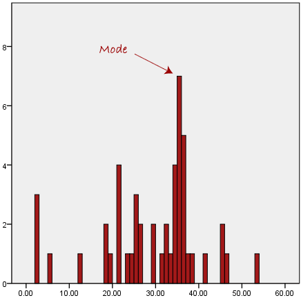
The mode is typically used for categorical data where we want to determine which category is the most common, as shown below:
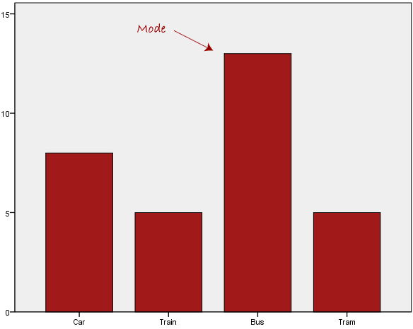
The bus is the most popular mode of transportation in this data set, as we can see above. However, because the mode is not unique, it causes problems when two or more values share the highest frequency, as shown below:
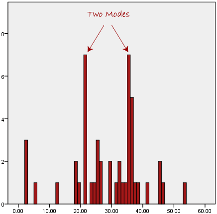
We're at a loss as to which mode best captures the data's central trend. When we have continuous data, this is especially problematic because we are less likely to have any one number that is more common than the others. Consider the following scenario: you're measuring the weight of 30 persons (to the nearest 0.1 kg). How often are we to discover two or more people that weigh precisely the same (for example, 67.4 kg)?
The answer is definitely quite doubtful - many people may be close, but with such a small sample (30 people) and such a wide range of possible weights, it's unlikely that you'll find two people who have exactly the same weight; that is, to the nearest 0.1 kg. This is why continuous data is rarely utilised with the mode.
Another issue with the mode is that when the most common mark is far away from the rest of the data in the data set, as shown in the graphic below, it will not offer us with a reliable estimate of central tendency.
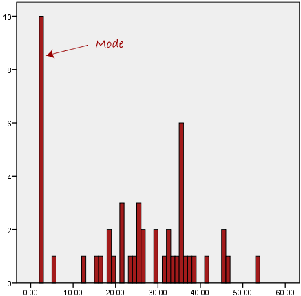
The mode has a value of 2 in the diagram above. The mean, on the other hand, is plainly not representative of the data, which is primarily concentrated in the 20 to 30 value range. It would be inaccurate to use the mode to describe the central tendency of this data collection.
Key takeaway
A single number that seeks to represent a set of data by identifying the centre position within that set of data is referred to as a measure of central tendency. As a result, central tendency measures are also known as central location measures.
Data dispersion is a term used to describe how data is distributed. It aids in the comprehension of data variance and offers information on data distribution. The methods used to understand the distribution data are range, IOR, variance, and standard deviation.
Data dispersion aids in the detection of outliers in a dataset.
Range
The range is the most straightforward data dispersion or measure of variability. By subtracting the lowest value from the enormous Number, the range can be calculated. The large range denotes great variability in the distribution, while the short range denotes low variability. Prepare all the values in ascending order, then subtract the lowest value from the highest value to determine a range.
Range = Highest_value – Lowest_value

The grade range is 18 points.
Outliers can have an impact on the range. If a range's value is affected by a single extreme value.

Variance
The term "variance" refers to a simple measure of dispersion. The variance of a dataset indicates how far each number deviates from the mean. Calculate the mean and squared deviations from the mean before calculating variance.
Population variation

Sample variance

The result is lower when the observation is close to the mean value, and higher when it is distant from the mean value.
Description of a variance formula with example
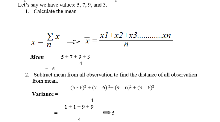
Mean deviation, Standard deviation
To obtain the original values, the standard deviation is the squared root of the variance. Data points with a low standard deviation are near to the mean.
The standard deviation is best understood with the help of the normal distribution.
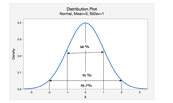
X indicates the mean value
68 % of values lie within 1 standard deviation.
95 % of values lies within 2 standard deviation.
99.7 % of values lie within 3 standard deviation.

By way of example, Standard deviation and Mean Absolute Deviation are defined (and why SD is more dependable than MAD).
Assume we have four values: 5, 7, 9, and 3.
1. Calculate the Mean:

2. To determine variance, subtract the mean from all observations to determine the distance between all values and the average (mean).

We recognised the outcome as zero since the identity features of a sample mean "deviation of a means is always sum to zero" whenever we discussed the mean.
As a result, we must work on it. We don't want any negative values in our system (as distance cannot be negative). We require a method for converting negative numbers to positive ones. We can use either mean absolute deviation or squared deviation as a measurement (Standard deviation).
Mean absolute deviation (MAD):
The MAD (Mean Absolute Deviation) is a measure of spread (variability).

Here, | denotes the absolute value, which means that all negative deviations (distances) are converted to positive values.
The issue with MAD is that it does not behave well as a squared deviation dosage in a normal distribution and is not differential. It is preferable to utilise squared deviation instead of MAD since squared deviation has well-defined mathematical features for normal distributions.
Key takeaway
Data dispersion is a term used to describe how data is distributed. It aids in the comprehension of data variance and offers information on data distribution. The methods used to understand the distribution data are range, IOR, variance, and standard deviation.
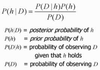
The posterior probability P(H|D) of a hypothesis is calculated as a product of the probability of the data given the hypothesis (P(D|H)), multiplied by the probability of the hypothesis (P(H)), divided by the probability of seeing the data, according to Bayes' Theorem. (P(D)) We've already seen one use of Bayes Theorem in class: in the analysis of Knowledge Cascades, we discovered that based on the conditional probabilities computed using Bayes' Theorem, reasonable decisions may be made where one's own personal information is omitted.
P(h/D) = P(D/h)P(h) / P(D)
By the law of product: P(h D) = P(h).P(D/h)
It's also commutative: P(D h) = P(D).P(h/D)
We can come up with the Bayesian formula as shown above if we combine them as equals. Also,
P(H) = Prior Probability.
P(D) = Likelihood of the data.
The Bayes' Theorem is the foundation of a form of Machine Learning known as Bayesian Machine Learning.
The Naive Bayes classifier is a tautological Bayesian Machine Learning technique that uses Bayes' Rule with the strong independence assumption that features in the dataset are conditionally independent of each other, given that we know the data class.
To comprehend Bayes Theorem in Machine Learning, it is necessary to comprehend that Bayes Theorem is quite useful in estimating value precision. Let's start at the beginning to understand how. The Bayes Theorem is a statement and theorem made by a British mathematician in the 18th century. He came up with a formula that works and is employed in conditional probability. What is conditional probability, exactly?
It's a phrase that refers to the likelihood of getting an answer to a question or predicting a likely outcome based on recent outcomes. A single statement is a method or process for cross-checking or updating existing forecasts in order to reduce the probability of making errors. In Machine Learning, this is how we express the Bayes Theorem.
Bayes' theorem is a mathematical formula for calculating the probability of an event based on ambiguous information. It is also known as Bayes' rule, Bayes' law, or Bayesian reasoning.
In probability theory, it relates the conditional and marginal probabilities of two random events.
The inspiration for Bayes' theorem came from British mathematician Thomas Bayes. Bayesian inference is a technique for applying Bayes' theorem, which is at the heart of Bayesian statistics.
It's a method for calculating the value of P(B|A) using P(A|B) knowledge.
Bayes' theorem can update the probability forecast of an occurrence based on new information from the real world.
Example: If cancer is linked to one's age, we can apply Bayes' theorem to more precisely forecast cancer risk based on age.
Bayes' theorem can be derived using the product rule and conditional probability of event A with known event B:
As a result of the product rule, we can write:
P(A ⋀ B)= P(A|B) P(B) or
In the same way, the likelihood of event B if event A is known is:
P(A ⋀ B)= P(B|A) P(A)
When we combine the right-hand sides of both equations, we get:
The above equation is known as Bayes' rule or Bayes' theorem (a). This equation is the starting point for most current AI systems for probabilistic inference.
It displays the simple relationship between joint and conditional probabilities. Here,
P(A|B) is the posterior, which we must compute, and it stands for Probability of hypothesis A when evidence B is present.
The likelihood is defined as P(B|A), in which the probability of evidence is computed after assuming that the hypothesis is valid.
Prior probability, or the likelihood of a hypothesis before taking into account the evidence, is denoted by P(A).
Marginal probability, or the likelihood of a single piece of evidence, is denoted by P(B).
In general, we can write P (B) = P(A)*P(B|Ai) in the equation (a), therefore the Bayes' rule can be expressed as:
Where A1, A2, A3,..... Is a set of mutually exclusive and exhaustive events, and An is a set of mutually exclusive and exhaustive events.
Use of Bayes’ Theorem
The purpose of doing an expert task, such as medical diagnosis, is to identify identifications (diseases) based on observations (symptoms). A relationship like this can be found in Bayes' Theorem.
P(A | B) = P(B | A) * P(A) / P(B)
Suppose: A=Patient has measles, B =has a rash
Then:P(measles/rash)=P(rash/measles) * P(measles) / P(rash)
Based on the known statistical values on the right, the desired diagnostic relationship on the left can be determined.
Applications of Bayes theorem
The theorem has a wide range of applications that aren't confined to finance. Bayes' theorem, for example, can be used to estimate the accuracy of medical test findings by taking into account how probable any specific person is to have a condition as well as the test's overall accuracy.
Key takeaway
Bayes' theorem, often known as Bayes' rule, Bayes' law, or Bayesian reasoning, is a mathematical formula for calculating the probability of an event based on ambiguous information.
The Bayesian inference is a method of applying Bayes' theorem, which is central to Bayesian statistics.
Hypothesis testing is a mathematical method for making statistical decisions based on evidence from experiments. Hypothesis testing is simply making an inference about a population parameter.
Hypothesis testing is the process of using statistical tests on a sample to draw inferences or conclusions about the overall population or data. T-test, which I will address in this tutorial, is used to draw the same inferences for various machine learning models.
We must make certain assumptions in order to draw some inferences, which leads to two concepts that are used in hypothesis testing.
● Null hypothesis: The null hypothesis refers to the belief that no anomaly trend occurs or to believing in the assumption made.
● Alternate hypothesis: Contrary to the null hypothesis, it indicates that observation is the result of a real effect.
P Values
It can also be used in machine learning algorithms as proof or a degree of significance for the null hypothesis. It is the value of the predictors in relation to the target.
In comparison, if the p-value in a machine learning model against an independent variable is less than 0.05, the variable is taken into account, implying that there is heterogeneous behavior with the target that is useful and can be learned by machine learning algorithms.
The following are the steps involved in hypothesis testing:
● Assume a null hypothesis; in most machine learning algorithms, no anomaly exists between the target and the independent variable.
● Obtain a sample
● Calculate the test results.
● Decide whether the null hypothesis should be accepted or rejected.
Error
Because of the scarcity of data resources, hypothesis testing is done on a sample of data rather than the entire population. Hypothesis testing can result in errors due to inferences drawn from sample data, which can be divided into two categories:
● Type I Error: We reject the null hypothesis when it is true in this error.
● Type II Error: We accept the null hypothesis when it is false in this error.
Hypothesis Testing's Importance
When you use statistics for data analytics, you start by making certain assumptions about how the data will be interpreted. These assumptions are frequently based on the premise that there are no relationships between variables. This is referred to as the "Null Hypothesis." The "Alternative Hypothesis," in contrast to the null hypothesis, is determined by comparing the p-value with the significance level or alpha. This p-value tells us whether or not we should take action. However, statistical errors known as type-1 and type-2 errors can arise while testing data, and they occur when the true null hypothesis is rejected or the false null hypothesis is accepted.
Key takeaway
Hypothesis testing is a mathematical method for making statistical decisions based on evidence from experiments. Hypothesis testing is simply making an inference about a population parameter.
The Pearson correlation method is the most widely used approach for numerical variables; it assigns a number between 0 and 1, with 0 representing no correlation, 1 representing total positive correlation, and 1 representing total negative correlation. This means that a correlation value of 0.7 between two variables indicates that there is a significant and positive association between them. A positive correlation indicates that if variable A rises, so will variable B, whereas a negative correlation indicates that if A rises, so will B.
The bivariate Pearson Correlation yields a sample correlation coefficient, r, that indicates the strength and direction of linear correlations between two continuous variables. By extension, the Pearson Correlation determines if statistical evidence exists for a linear relationship between the same pairs of variables in the population, as indicated by a population correlation coefficient ("rho"). A parametric measure is the Pearson Correlation.
This metric is also referred to as:
● Pearson’s correlation
● Pearson product-moment correlation (PPMC)
Uses
The bivariate Pearson Correlation is frequently used to assess:
● Correlations between two variables.
● Within and between sets of variables, there are correlations.
The Pearson bivariate correlation reveals the following:
● Whether two continuous variables have a statistically significant linear connection.
● A linear relationship's strength (i.e., how close the relationship is to being a perfectly straight line).
● A linear relationship's direction (increasing or decreasing).
Non-linear correlations and relationships between categorical variables are not addressed by the bivariate Pearson Correlation. You'll need to use a different measure of association if you want to comprehend links including categorical variables and/or non-linear relationships.
Only relationships between continuous variables are revealed by the bivariate Pearson Correlation. No matter how large the correlation coefficient is, the bivariate Pearson Correlation does not yield any judgments about causality.
Key takeaway
The Pearson correlation method is the most widely used approach for numerical variables; it assigns a number between 0 and 1, with 0 representing no correlation, 1 representing total positive correlation, and 1 representing total negative correlation.
The sample correlation coefficient between two variables x and y is denoted by the letters r or rxy and is calculated as follows:
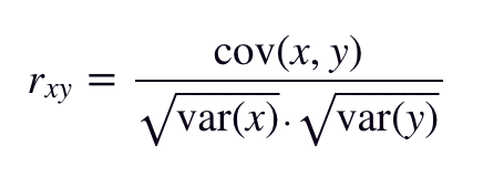
Where cov(x, y) represents the sample covariance of x and y, var(x) represents the sample variance of x, and var(y) represents the sample variance of y.
Correlation can have any value between -1 and 1. The magnitude of the correlation (how close it is to -1 or +1) reflects the intensity of the relationship, whereas the sign of the correlation coefficient indicates the direction of the association.
● -1: perfectly negative linear relationship
● 0: no relationship
● +1: perfectly positive linear relationship
These general parameters (which may vary by discipline) can be used to judge strength:
● .1 < | r | < .3 … small / weak correlation
● .3 < | r | < .5 … medium / moderate correlation
● .5 < | r | ……… large / strong correlation
A correlation's direction and strength are two separate qualities. Correlations with r = +0.90, r = 0.00, and r = -0.90 are shown in the scatterplots below. The nonzero correlations have the same strength: 0.90. However, the correlations are not in the same direction: a negative correlation indicates a decreasing link, whereas a positive correlation indicates a rising association.
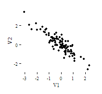
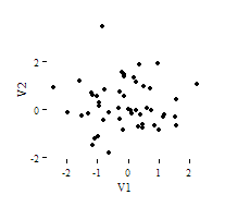
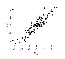
In this graph, there is no discernible growing or diminishing linear trend for the r = 0.00 correlation. Keep in mind, however, that Pearson correlation can only discover linear correlations, thus a pair of variables with a high nonlinear link and a tiny Pearson correlation coefficient is possible. Making scatterplots of your variables to verify your correlation coefficients is a smart idea.
The Chi-Square Test of Independence analyses whether categorical variables are associated (i.e., whether the variables are independent or related). It's a test that isn't parametric.
This test is also referred to as: Chi-Square Test of Association.
The data is analysed using a contingency table in this test. A contingency table (sometimes called a cross-tabulation, crosstab, or two-way table) is a data classification system that uses two categorical variables. One variable's categories appear in rows, while the other variable's categories appear in columns. There must be two or more categories for each variable. The total number of cases for each pair of categories is represented in each cell.
Types
The Chi-square test is used to determine whether your data is as expected. The test's core premise is to compare the observed values in your data to the expected values that you would see if the null hypothesis is true.
The Chi-square goodness of fit test and the Chi-square test of independence are two regularly used Chi-square tests. Both tests use variables to categorise your data into groups. As a result, people may be unsure which test they should use. The two tests are compared in the table below.
Examples, as well as explanations on assumptions and computations, can be found on the specific pages for each type of Chi-square test.
Table 1: Choosing a Chi-square test
| Chi-Square Goodness of Fit Test | Chi-Square Test of Independence |
Number of variables | One | Two |
Purpose of test | Determine whether or not one variable is likely to originate from a given distribution. | Determine whether two variables are connected or unrelated. |
Example | Determine whether each type of candy has the same amount of pieces in each bag. | Determine whether moviegoers' snack purchases are related to the type of film they intend to watch. |
Hypotheses in example | H0: The proportion of candy flavours is the same. Ha: The flavour proportions aren't the same.
| H0: The proportion of people who buy snacks is unaffected by the sort of film. Ha: For different sorts of movies, the proportion of individuals who buy snacks varies. |
Theoretical distribution used in test | Chi-Square | Chi-Square |
Degrees of freedom | 1 less than the total number of categories. In our example, the number of candy flavours minus one | Number of categories for first variable minus 1, multiplied by number of categories for second variable minus 1. In our example, number of movie categories minus 1, multiplied by 1 (because snack purchase is a Yes/No variable and 2-1 = 1) |
How to perform a Chi-square test
You execute the identical analysis steps for the Chi-square goodness of fit test and the Chi-square test of independence, which are listed below. To see these steps in action, go to the pages for each type of exam.
● Before you start collecting data, define your null and alternative hypotheses.
● Make a decision on the alpha value. This entails deciding how much of a chance you're willing to take on the possibility of coming to the wrong decision. Let's say you want to test for independence with a value of 0.05. You've decided to take a 5% chance of concluding that the two variables are independent when they aren't.
● Check for any inaccuracies in the data.
● Examine the test's assumptions. (For further information on assumptions, see the pages for each test type.)
● Carry out the test and come to a conclusion.
Calculating a test statistic is required for both Chi-square tests in the table above. The tests are designed to compare actual data values to what would be predicted if the null hypothesis is true. Finding the squared difference between actual and expected data values and dividing that difference by the expected data values is the test statistic. You repeat this process for each data point and total the results.
The test statistic is then compared to a theoretical value from the Chi-square distribution. The theoretical value is determined by the data's alpha value and degrees of freedom.
Key takeaway
The Chi-Square Test of Independence analyses whether categorical variables are associated (i.e., whether the variables are independent or related). It's a test that isn't parametric.
T-tests are often used in statistics and econometrics to determine whether two outcomes or variables have different values.
The scale of measurement, random sampling, normality of data distribution, adequacy of sample size, and equality of variance in standard deviation are all frequent assumptions made when doing a t-test.
The goal of parametric testing is to provide a statistical inference about the population by performing statistically significant tests (such as the t-test) on a sample taken from the population. The t-test is a parametric test based on a student's t statistic. This statistic is based on the assumption that variables are selected from a typical population. In this t-test statistic, the population mean has been assumed to be known. The t-distribution has a bell-shaped look, similar to that of a normal distribution.
Statistics Solutions is a leader in statistical consulting and t-test analysis in the United States.
A chemist working for the Guinness brewing company devised the t-test as a straightforward technique to assess the consistency of stout quality. 1 It was refined and adapted, and it currently refers to any statistical hypothesis test in which the statistic being evaluated is predicted to correlate to a t-distribution if the null hypothesis is true.
A t-test is a statistical assessment of two population means; a two-sample t-test is typically employed with small sample sizes to examine the difference between the samples when the variances of two normal distributions are unknown.
T-Test Assumptions
● The first assumption made about t-tests is about the measuring scale. A t-test assumes that the scale of measurement applied to the data obtained is on a continuous or ordinal scale, such as the results of an IQ test.
● The second assumption is that the data is taken from a representative, randomly selected fraction of the overall population, as in a basic random sample.
● The third assumption is that the data produces a normal distribution, bell-shaped distribution curve when plotted. When a normal distribution is assumed, a condition for acceptance can be specified as a level of probability (alpha level, level of significance, p). In the vast majority of circumstances, a 5% value can be accepted.
● The fourth assumption is that the sample size is large enough. With a higher sample size, the results distribution should resemble a regular bell-shaped curve.
● The final assumption is variance homogeneity. When the standard deviations of samples are almost equal, homogeneous, or equal, variance exists.
Key takeaway
A t-test is a statistical tool for determining if the means of two groups differ significantly based on a sample of data.
For the test to be properly evaluated and valid, it must be based on a set of assumptions.
The data must be randomly collected from the population of interest, and the data variables must have a normal distribution, among other assumptions.
References:
- David Dietrich, Barry Hiller, “Data Science and Big Data Analytics”, EMC education services, Wiley publication, 2012, ISBN0-07-120413-X
- DT Editorial Services, “Big Data, Black Book”, DT Editorial Services, ISBN:
9789351197577, 2016 Edition
3. Wes McKinney, “Python for Data Analysis”, O' Reilly media, ISBN: 978-1-449-31979-3