Unit - 4
Predictive Big Data Analytics with Python
Predictive modelling is usually a pleasurable experience. The majority of your work will be spent determining what the firm need and then framing your challenge. The next stage is to customise the solution to the client's requirements. As we solve more problems, we realise that we can use a framework to create our first cut models. This framework not only helps you get faster results, but it also helps you prepare for the following stages depending on the outcomes.
Using past data, predictive analysis provides predictions about what might happen in the future. The information is gathered in a basetable that has three key components: population, candidate predictors, and target. The population is the set of persons or things for which you want to make predictions. Candidate predictors are people or items in a population who, given certain knowledge, could be used to forecast an event. Finally, the target has information about the events to predict. It is one if events occur, and zero otherwise.
In this predictive analysis, we'll look at a non-profit organisation that has a donor database containing people who have donated previously. This organisation is considering writing to its donors and asking them to donate to a specific project.
● Sending the letter to all of the candidate contributors is one possibility. However, this might be quite costly.
● We can use predictive analysis to identify the donors who are most likely to donate.
Python is a multi-purpose programming language that is frequently used for purposes other than data analysis and data science. What makes Python so handy for data manipulation?
There are libraries that provide users with the capabilities they require when processing data. The key Python libraries for working with data are listed below. You should spend some time learning about the basic functions of these programmes.
Numpy and Scipy – Fundamental Scientific Computing
Numerical Python is referred to as NumPy. The n-dimensional array is NumPy's most powerful feature. Basic linear algebra operations, Fourier transforms, additional random number capabilities, and tools for integration with other low-level languages like Fortran, C, and C++ are also included in this package.
Scientific Python (SciPy) is a Python programming language. It is based on the NumPy programming language. Scipy is a handy library for a wide range of high-level science and engineering modules, including discrete Fourier transforms, linear algebra, optimization, and sparse matrices.
Pandas – Data Manipulation and Analysis
Pandas is a programming language that may be used to do structured data operations and manipulations. It's often used for data preprocessing and munging. Pandas were just recently added to Python, but they've already helped to increase Python's popularity among data scientists.
Matplotlib – Plotting and Visualization
Matplotlib may be used to plot a wide range of graphs, from histograms to line plots to heat plots. To use these charting features inline, use the Pylab feature in ipython notebook (ipython notebook –pylab = inline). If you don't use the inline option, pylab turns the ipython environment to a Matlab-like environment.
Scikit-learn – Machine Learning and Data Mining
For machine learning, use Scikit Learn. This library, which is based on NumPy, SciPy, and Matplotlib, includes a number of useful tools for machine learning and statistical modelling, such as classification, regression, clustering, and dimensional reduction.
StatsModels – Statistical Modeling, Testing, and Analysis
Statsmodels is a statistical modelling software package. It's a Python package that lets you look at data, estimate statistical models, and run statistical tests. For various types of data and each estimator, a comprehensive array of descriptive statistics, statistical tests, charting functions, and outcome statistics is offered.
Seaborn – For Statistical Data Visualization
Seaborn is a tool for visualising statistical data. It's a Python module for creating visually appealing and useful statistics visuals. It is based on the matplotlib library. Seaborn aspires to make visualisation a key component of data exploration and comprehension.
Now that you've discovered that the dataset contains duplicates, you'll want to get rid of them. You can get rid of duplicates in two methods. The first deletes all of the rows, whereas the second deletes the column with the most duplicates.
Method 1: Remove the values from all duplicate rows.
Using the drop duplicates function, you can remove all rows with the same values ().
Data_obj.drop_duplicates()
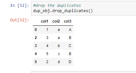
It will delete all duplicate values from the dataset, leaving just unique values.
Method 2: Remove the duplicates from the columns that have the most of them.
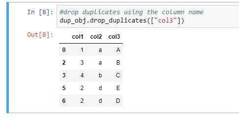
Instead of eliminating the full row's value, you'll remove the column with the most duplicated values using this method.
Drop_duplicates([colum_list])
Assuming that col3 has more duplicates than the other columns in this example, I will just use the procedure to eliminate this column.
Data_obj.drop_duplicates(["col3"])
We learned how to merge data from several sources into a single dataframe. We now have a large number of columns with various types of data. Our goal is to convert the data into a format that machine learning can understand. All machine learning algorithms are mathematically grounded. As a result, all of the columns must be converted to numerical format. Let's have a look at the various forms of data we have.
In a larger sense, data is divided into numerical and category categories:
Numerical: As the name suggests, this is numeric data that is quantifiable.
Categorical: The data is a string or non-numeric data that is qualitative in nature.
The following categories are used to categorise numerical data:
Discrete: To explain in simple terms, any numerical data that is countable is called discrete, for example, the number of people in a family or the number of students in a class. Discrete data can only take certain values (such as 1, 2, 3, 4, etc).
Continuous: Any numerical data that is measurable is called continuous, for example, the height of a person or the time taken to reach a destination. Continuous data can take virtually any value (for example, 1.25, 3.8888, and 77.1276).
The Transform function in Pandas (Python) can be a little confusing at first, particularly if you're coming from an Excel background. To be honest, most data scientists don't use it immediately away in their training.
However, as a data scientist, Pandas' transform function is quite useful! It's a powerful feature engineering function in Python that you can rely on.
After applying the function specified in its parameter, Python's Transform function returns a self-produced dataframe with transformed values. The length of this dataframe is the same as the passed dataframe.
That was a lot to take in, so let me give you an example.
Assume we wish to multiply each element in a dataframe by 10:
#import library
Import pandas as pd
Import numpy as np
#creating a dataframe
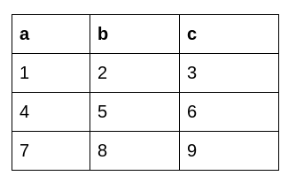
Df=pd.DataFrame(np.array([[1, 2, 3], [4, 5, 6], [7, 8, 9]]), columns=['a', 'b', 'c'])
The original data frame looks like this:
#applying the transform function
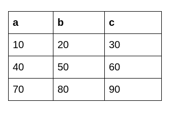
Df.transform(func = lambda x : x * 10)
After using Python's Transform function, we get the following dataframe:
Missing data in the training data set might diminish a model's power / fit, or lead to a biassed model if the behaviour and relationships with other variables are not properly analysed. It can lead to incorrect classification or prediction.
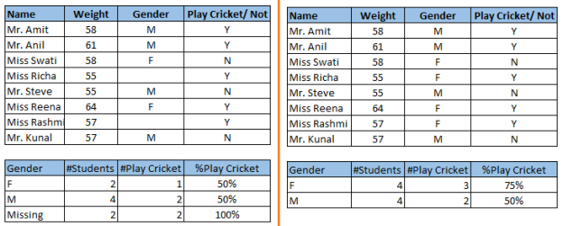
In the figure above, take note of the missing values: We haven't dealt with missing values in the left situation. The conclusion drawn from this data set is that males have a better chance of playing cricket than ladies. On the other hand, the second table, which presents data after missing values have been treated (depending on gender), demonstrates that girls have a larger chance of playing cricket than males.
Why does my data have missing values?
We looked at how missing values in a dataset should be handled. Let's look into the causes of these missing values. They can happen in two stages:
Data Extraction: It's conceivable that the extraction process is having issues. In such circumstances, we should double-check the data with data guardians to ensure that it is correct. To ensure that data extraction is valid, certain hashing algorithms can be utilised. Errors in the data extraction stage are usually easy to spot and remedy.
Data collection: These errors occur throughout the data collection process and are more difficult to fix. They are divided into four categories:
● Missing completely at random: The chance of a missing variable is the same for all observations in this situation. For example, after flipping a fair coin, respondents to a data collection process elect to reveal their earnings. In the event of a head, the respondent reports his or her earnings, and vice versa. Each observation has the same chance of having a missing value.
● Missing at random: When a variable becomes missing at random, the missing ratio fluctuates depending on the values / levels of the other input variables. For instance, we're gathering age data, and females have a greater missing value than males.
● Missing that depends on unobserved predictors: The missing values are not random and are related to the unobserved input variable in this scenario. For example, in a medical study, if a certain diagnosis causes discomfort, the study's participants are more likely to drop out. Unless we have added "discomfort" as an input variable for all patients, this missing value is not random.
● Missing that depends on the missing value itself: This is a situation in which the chance of a missing value is proportional to the value itself. People with higher or lower income, for example, are more inclined to provide non-response to their earnings.
Strategies for dealing with missing values
Deletions: List Wise Deletion and Pair Wise Deletion are the two types of deletion.
● We eliminate observations where any of the variables is missing in list wise deletion. One of the key advantages of this strategy is its simplicity; nevertheless, because the sample size is reduced, it limits the model's power.
● We undertake analysis for all situations in which the variables of interest are present in pair wise deletion. This strategy has the advantage of keeping as many examples available for study as possible. One of the method's drawbacks is that various sample sizes are used for different variables.
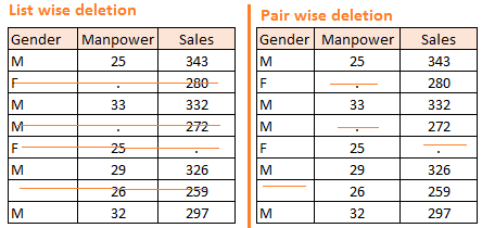
● When the nature of missing data is "Missing fully at random," deletion methods are applied; otherwise, non-random missing values can bias the model output.
Mean/ Mode/ Median Imputation: Imputation is a technique for replacing missing values with estimates. The goal is to use known associations that can be found in the valid values of the data set to help estimate the missing values. One of the most commonly used approaches is mean, mode, and median imputation. It consists of substituting missing data for a particular property with the mean, median, or mode (quantitative attribute) of all known values for that variable. It can be one of two kinds:
● Generalized Imputation: In this scenario, the mean or median for all non-missing values of that variable is calculated, and the missing value is replaced with the mean or median. Because variable "Manpower" is missing in the table above, we take the average of all non-missing values of "Manpower" (28.33) and use it to replace the missing value.
● Similar case Imputation: In this situation, we calculate the average of non-missing values for the genders "Male" (29.75) and "Female" (25) separately, then replace the missing value based on gender. We'll use 29.75 in place of missing manpower values for "Male" and 25 in place of missing manpower values for "Female."
Prediction model: One of the more complex methods for dealing with missing data is to use a prediction model. In this step, we develop a predictive model to estimate values that will be used to fill in the gaps in the data. In this scenario, we split our data into two groups: one with no missing values for the variable and one with missing values. The first data set is used as the model's training data set, while the second data set with missing values is used as the model's test data set, and the variable with missing values is considered as the target variable. Then, using other properties from the training data set, we build a model to predict the target variable and fill in missing values in the test data set. To do so, we can use regression, ANOVA, logistic regression, and other modelling techniques. This strategy has two disadvantages:
● The estimated values of the model are frequently better behaved than the genuine ones.
● The model will not be precise for estimating missing values if there are no links between characteristics in the data set and the attribute with missing values.
KNN Imputation: The missing values of an attribute are imputed using the supplied number of attributes that are most comparable to the attribute whose values are missing in this method of imputation. A distance function is used to determine the similarity of two properties. It is also known to have some benefits and drawbacks.
Advantages:
● Both qualitative and quantitative traits can be predicted using k-nearest neighbour.
● It is not necessary to create a predictive model for each attribute with incomplete data.
● Multiple missing values in an attribute can be readily treated.
● The data's correlation structure is taken into account.
Disadvantages:
● When studying a huge database, the KNN method takes a long time. It looks for the most comparable instances across the entire dataset.
● The k-value you choose is really important. A higher k number would include features that are notably different from what we require, whereas a lower k value would indicate that major attributes are lacking.
The problem of dealing with outliers follows that of dealing with missing values. When developing models, we frequently overlook outliers. This is a demoralising behaviour. Outliers tend to bias your data, lowering its accuracy. Let's take a closer look into outlier therapy.
The discovery and transmission of important patterns in data is what analytics is all about. Analytics focuses on the simultaneous application of statistics, computer programming, and operation research to qualify performance, which is especially useful in sectors with a lot of recorded data. When it comes to communicating insights, data visualisation is frequently used.
Analytics is frequently used by businesses to describe, forecast, and enhance business performance. Predictive analytics, enterprise decision management, and other areas in particular are covered. Because analytics can need a lot of processing (due to massive data), the algorithms and tools utilised in analytics use the most up-to-date computer science methodologies.
In a word, analytics is the scientific process of turning data into knowledge in order to make better judgments. The purpose of data analytics is to obtain actionable insights that lead to better business decisions and outcomes.
There are three types of data analytics:
● Predictive (forecasting)
● Descriptive (business intelligence and data mining)
● Prescriptive (optimization and simulation)
Predictive analytics
Predictive analytics transforms data into useful, actionable data. Data is used in predictive analytics to anticipate the likely outcome of an event or the likelihood of a condition occurring.
Predictive analytics encompasses a wide range of statistical approaches including modelling, machine learning, data mining, and game theory, all of which examine current and historical data to create predictions about the future. The following are some of the techniques used in predictive analytics:
● Linear Regression
● Time series analysis and forecasting
● Data Mining
There are three basic cornerstones of predictive analytics:
● Predictive modeling
● Decision Analysis and optimization
● Transaction profiling
Descriptive analytics
Descriptive analytics examines data and analyses previous events in order to provide insight into how to approach future events. It analyses and comprehends prior performance by mining historical data to determine what caused success or failure in the past. This form of analysis is used in almost all management reporting, including sales, marketing, operations, and finance.
The descriptive model quantifies data relationships in a way that is frequently used to group consumers or prospects. Unlike predictive models, which focus on predicting the behaviour of a particular consumer, descriptive analytics discovers a variety of customer-product correlations.
Descriptive analytics is commonly used in company reports that provide historical reviews, such as:
● Data Queries
● Reports
● Descriptive Statistics
● Data dashboard
Prescriptive analytics
Prescriptive analytics automatically combines big data, mathematics, business rules, and machine learning to produce a forecast and then provides a decision alternative to capitalise on the prediction.
Prescriptive analytics goes beyond forecasting future events by recommending actions based on the predictions and displaying the implications of each decision option to the decision maker. Prescriptive analytics predicts not just what will happen and when it will happen, but also why. Prescriptive Analytics can also provide decision options for how to capitalise on a future opportunity or avoid a future danger, as well as illustrate the implications of each option.
Prescriptive analytics, for example, can assist healthcare strategic planning by combining operational and utilisation data with data from external sources such as economic data, population demography, and so on.
The Apriori Algorithm is a Machine Learning algorithm for gaining insight into the hierarchical relationships between the many things involved. The algorithm's most common practical application is to recommend purchases based on the items already in the user's cart. Walmart, in particular, has made extensive use of the algorithm to recommend products to its customers.
Any subset of a frequent itemset must be frequent, according to the apriori method.

For example, a transaction that includes wine, chips, and bread also includes wine and bread. So, if wine, chips, and bread are common, then wine, bread must likewise be common, according to the Apriori principle.
Limitations
Despite its simplicity, Apriori algorithms have a number of drawbacks, including:
● When dealing with a huge number of candidates with frequent itemets, it's a waste of time.
● When a large number of transactions are processed through a limited memory capacity, the efficiency of this algorithm suffers.
● It was necessary to use a lot of computing power and to scan the entire database.
Improvements
The following are some suggestions for increasing the algorithm's efficiency:
● Reduce the number of database scans by using hashing algorithms.
● Don't think about the infrequent transaction any more.
● If a purchase is common in one division, it should also be common in another.
● To improve the accuracy of your algorithm, select random samples.
● While the database is being scanned, use dynamic itemset counting to add new candidate itemsets.
Applications
The algorithm is used in a variety of ways, including:
● Forest agencies use it to figure out how intense and likely forest fires are.
● Auto-complete functions are used by Google and other search engines.
● Such algorithms were employed by the healthcare department to assess the patient information and predict which people would acquire high blood pressure, diabetes, or another common condition.
● To increase academic success, students are classified into groups depending on their specialties and performance.
● To deliver a better user experience, e-commerce websites integrate it in their recommendation algorithms.
Implementation of algorithm in Python
Step 1: Importing the essential libraries is the first step.
Import numpy as np
Import pandas as pd
From mlxtend.frequent_patterns import apriori, association_rules
Step 2: Data loading and exploration
# Changing the working location to the location of the file
Cd C:\Users\Dev\Desktop\Kaggle\Apriori Algorithm
# Loading the Data
Data = pd.read_excel('Online_Retail.xlsx')
Data.head()

# Exploring the columns of the data
Data.columns

Step 3: Cleaning the Data
# Stripping extra spaces in the description
Data['Description'] = data['Description'].str.strip()
# Dropping the rows without any invoice number
Data.dropna(axis = 0, subset =['InvoiceNo'], inplace = True)
Data['InvoiceNo'] = data['InvoiceNo'].astype('str')
# Dropping all transactions which were done on credit
Data = data[~data['InvoiceNo'].str.contains('C')]
Step 4: Dividing the data into regions based on the transaction.
# Transactions done in France
Basket_France = (data[data['Country'] =="France"]
.groupby(['InvoiceNo', 'Description'])['Quantity']
.sum().unstack().reset_index().fillna(0)
.set_index('InvoiceNo'))
# Transactions done in the United Kingdom
Basket_UK = (data[data['Country'] =="United Kingdom"]
.groupby(['InvoiceNo', 'Description'])['Quantity']
.sum().unstack().reset_index().fillna(0)
.set_index('InvoiceNo'))
# Transactions done in Portugal
Basket_Por = (data[data['Country'] =="Portugal"]
.groupby(['InvoiceNo', 'Description'])['Quantity']
.sum().unstack().reset_index().fillna(0)
.set_index('InvoiceNo'))
Basket_Sweden = (data[data['Country'] =="Sweden"]
.groupby(['InvoiceNo', 'Description'])['Quantity']
.sum().unstack().reset_index().fillna(0)
.set_index('InvoiceNo'))
Step 5: Data encoding on the fly
# Defining the hot encoding function to make the data suitable
# for the concerned libraries
Def hot_encode(x):
If(x<= 0):
Return 0
If(x>= 1):
Return 1
# Encoding the datasets
Basket_encoded = basket_France.applymap(hot_encode)
Basket_France = basket_encoded
Basket_encoded = basket_UK.applymap(hot_encode)
Basket_UK = basket_encoded
Basket_encoded = basket_Por.applymap(hot_encode)
Basket_Por = basket_encoded
Basket_encoded = basket_Sweden.applymap(hot_encode)
Basket_Sweden = basket_encoded
Step 6: Create the models and analyse the outcomes.
Have you ever gone to a search engine and typed in a word or a portion of a word, only to have the search engine complete the search term for you? Perhaps it suggested something you were unaware of and you went looking for it instead. This necessitates a method for quickly locating frequently used itemsets. By storing the dataset in a particular structure called an FP-tree, the FP-growth method finds frequent itemsets or pairings, or groupings of things that frequently occur together.
Han proposed the FP-Growth Algorithm in, which is an efficient and scalable method for mining the entire set of frequent patterns by pattern fragment growth, using an extended prefix-tree structure for storing compressed and crucial information about frequent patterns called the frequent-pattern tree (FP-tree). Han demonstrated that his method surpasses other prominent methods for mining frequent patterns, such as the Apriori Algorithm and TreeProjection, in his research.
Only twice is the dataset scanned by the FP-growth algorithm. The following is the fundamental way to utilise the FP-growth algorithm to find common itemsets:
1st, construct the FP-tree.
2 Mine itemsets from the FP-tree on a regular basis.
"Frequent pattern" is abbreviated as FP. An FP-tree resembles other computer science trees, except it contains links that connect comparable things. A linked list can be made up of the linked items.
The FPtree is a data structure for storing the frequency of occurrence of objects in groups. Paths are used to store sets.
In the canopy of the tree Part of the tree will be shared by sets with related items. The tree will only split when they disagree. A node represents a single item from the set, as well as the number of times it appeared in the sequence. The number of times a sequence occurred is indicated by a path.
Node linkages, or links between similar items, will be utilised to find the location of comparable items quickly.
FP-growth algorithm
Pros: Apriori is usually faster.
Cons: Difficult to implement; performance degrades with certain datasets.
Nominal values are used.
General approach to FP-growth algorithm
Collecting can be done in a variety of ways.
Because we're storing sets, we'll require discrete data. Continuous data must be quantized into discrete values if it is to be used.
Analyze: Any technique.
Train by constructing an FP-tree and mining it.
Doesn't apply in this case.
Use: This can be used to find often occurring objects that can be utilised to make decisions, recommend items, forecast, and so on.
A powerful statistical analysis tool is regression analysis. The values of additional independent variables in a data collection are predicted using a dependent variable of our interest.
We come with regression on a regular basis in an intuitive sense. Predicting the weather using a data set of previous weather conditions is an example.
To analyse and predict the outcome, it employs a variety of approaches, although the focus is mostly on the relationship between the dependent variable and one or more independent variables.
The outcome of a binary variable with only two possible outcomes is predicted using logistic regression analysis.
Linear regression
It's a method for analysing a data set with a dependent variable and one or more independent variables in order to predict the outcome of a binary variable, which has only two possibilities.
Categorical is the kind of the dependent variable. The goal variable is also known as the dependent variable, and the predictors are the independent variables.
Logistic regression is a type of linear regression in which just the outcome of a categorical variable is predicted. The log function is used to predict the probability of an event.
To forecast the category value, we employ the Sigmoid function/curve. The outcome (win/loss) is determined by the threshold value.
Linear regression equation: y = β0 + β1X1 + β2X2 …. + βnXn
● The dependent variable that has to be predicted is denoted by the letter Y.
● The Y-intercept, or point on the line that contacts the y-axis, is equal to 0.
● The slope of the line is 1. (the slope can be negative or positive depending on the relationship between the dependent variable and the independent variable.)
● The independent variable utilised to predict our resultant dependent value is denoted by the letter X.
Sigmoid function: p = 1 / 1 + e-y
Apply the sigmoid function on the linear regression equation.
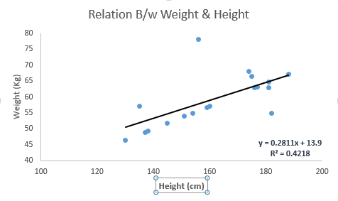
● The independent and dependent variables must have a linear relationship.
● Multicollinearity, autocorrelation, and heteroskedasticity are all problems with multiple regression.
● Outliers are particularly sensitive in linear regression. It can have a significant impact on the regression line and, as a result, the anticipated values.
● Multicollinearity can increase the variance of coefficient estimates, making them extremely sensitive to slight model modifications. As a result, the coefficient estimations are insecure.
● We can use a forward selection, backward elimination, or stepwise strategy to select the most significant independent variables when there are several independent variables.
Logistic regression
The likelihood of event=Success and event=Failure is calculated using logistic regression. When the dependent variable is binary (0/ 1, True/ False, Yes/ No), we should apply logistic regression. The value of Y here ranges from 0 to 1, and it can be represented using the equation below.
Odds= p/ (1-p) = probability of event occurrence / probability of not event occurrence
Ln(odds) = ln(p/(1-p))
Logit(p) = ln(p/(1-p)) = b0+b1X1+b2X2+b3X3....+bkXk
The likelihood of the presence of the characteristic of interest, p, is given above. "Why have we utilised log in the equation?" is a question you should ask.
We need to find a link function that is best suited for a binomial distribution (dependent variable) because we are working with one. It's also a logit function. Instead of minimising the sum of squared errors, the parameters in the equation above are set to increase the chances of witnessing the sample values (like in ordinary regression).
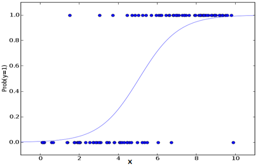
● For classification difficulties, logistic regression is commonly employed.
● There is no requirement for a linear relationship between the dependent and independent variables in logistic regression. Because it uses a non-linear log transformation on the anticipated odds ratio, it can handle a wide range of relationships.
● All major factors should be included to avoid overfitting and underfitting. Using a step-by-step procedure to estimate the logistic regression is a smart way to ensure this behaviour.
● Because maximum likelihood estimates are less powerful than ordinary least squares estimates for small sample sizes, it necessitates large sample sizes.
● There should be no correlation between the independent variables, i.e. no multicollinearity. However, we have the option of include categorical variable interaction effects in the study and model.
● Ordinal logistic regression is used when the values of the dependent variable are ordinal.
● Multinomial Logistic regression is used when the dependent variable has multiple classes.
The Naïve Bayes algorithm is comprised of two words Naïve and Bayes, Which can
Be described as:
● Naïve: It is called Naïve because it assumes that the occurrence of a certain feature is independent of the occurrence of other features. Such as if the fruit is identified based on color, shape, and taste, then red, spherical, and sweet fruit is recognized as an apple. Hence each feature individually contributes to identifying that it is an apple without depending on each other.
● Bayes: It is called Bayes because it depends on the principle of Bayes’ Theorem.
Naïve Bayes Classifier Algorithm
Naïve Bayes algorithm is a supervised learning algorithm, which is based on the
Bayes theorem and used for solving classification problems. It is mainly used in text
Classification that includes a high-dimensional training dataset.
Naïve Bayes Classifier is one of the simple and most effective Classification algorithms which help in building fast machine learning models that can make quick predictions.
It is a probabilistic classifier, which means it predicts based on the probability of an
Object.
Some popular examples of the Naïve Bayes Algorithm are spam filtration,
Sentimental analysis, and classifying articles.
Bayes’ Theorem:
● Bayes’ theorem is also known as Bayes’ Rule or Bayes’ law, which is used to determine the probability of a hypothesis with prior knowledge. It depends on the conditional probability.
● The formula for Bayes’ theorem is given as:

Where,
● P(A|B) is Posterior probability: Probability of hypothesis A on the observed event B.
● P(B|A) is Likelihood probability: Probability of the evidence given that the probability of a hypothesis is true.
● P(A) is Prior Probability: Probability of hypothesis before observing the evidence.
● P(B) is a Marginal Probability: Probability of Evidence.
Working of Naïve Bayes’ Classifier can be understood with the help of the below example:
Suppose we have a dataset of weather conditions and corresponding target variable
“Play”. So using this dataset we need to decide whether we should play or not on a
Particular day according to the weather conditions. So to solve this problem, we need to follow the below steps:
Convert the given dataset into frequency tables.
Generate a Likelihood table by finding the probabilities of given features.
Now, use Bayes theorem to calculate the posterior probability.
Problem: If the weather is sunny, then the Player should play or not?
Solution: To solve this, first consider the below dataset:
Outlook Play
0 Rainy Yes
1 Sunny Yes
2 Overcast Yes
3 Overcast Yes
4 Sunny No
5 Rainy Yes
6 Sunny Yes
7 Overcast Yes
8 Rainy No
9 Sunny No
10 Sunny Yes
11 Rainy No
12 Overcast Yes
13 Overcast Yes
Frequency table for the Weather Conditions:
Weather Yes No
Overcast 5 0
Rainy 2 2
Sunny 3 2
Total 10 5
Likelihood table weather condition:
Weather No Yes
Overcast 0 5 5/14 = 0.35
Rainy 2 2 4/14 = 0.29
Sunny 2 3 5/14 = 0.35
All 4/14=0.29 10/14=0.71
Applying Bayes’ theorem:
P(Yes|Sunny)= P(Sunny|Yes)*P(Yes)/P(Sunny)
P(Sunny|Yes)= 3/10= 0.3
P(Sunny)= 0.35
P(Yes)=0.71
So P(Yes|Sunny) = 0.3*0.71/0.35= 0.60
P(No|Sunny)= P(Sunny|No)*P(No)/P(Sunny)
P(Sunny|NO)= 2/4=0.5
P(No)= 0.29
P(Sunny)= 0.35
So P(No|Sunny)= 0.5*0.29/0.35 = 0.41
So as we can see from the above calculation that P(Yes|Sunny)>P(No|Sunny)
Hence on a Sunny day, the Player can play the game.
Advantages of Naïve Bayes Classifier:
● Naïve Bayes is one of the fast and easy ML algorithms to predict a class of datasets.
● It can be used for Binary as well as Multi-class Classifications.
● It performs well in Multi-class predictions as compared to the other Algorithms.
● It is the most popular choice for text classification problems.
Disadvantages of Naïve Bayes Classifier:
● Naive Bayes assumes that all features are independent or unrelated, so it cannot learn the relationship between features.
Applications of Naïve Bayes Classifier:
● It is used for Credit Scoring.
● It is used in medical data classification.
● It can be used in real-time predictions because Naïve Bayes Classifier is an eager
● learner.
● It is used in Text classification such as Spam filtering and Sentiment analysis.
Types of Naïve Bayes Model:
There are three types of Naive Bayes Model, which are given below:
Gaussian: The Gaussian model assumes that features follow a normal distribution.
This means if predictors take continuous values instead of discrete, then the model
Assumes that these values are sampled from the Gaussian distribution.
Multinomial: The Multinomial Naïve Bayes classifier is used when the data is
Multinomial distributed. It is primarily used for document classification problems, it
Means a particular document belongs to which category such as Sports, Politics,
Education, etc.
The classifier uses the frequency of words for the predictors.
Bernoulli: The Bernoulli classifier works similarly to the Multinomial classifier, but the predictor variables are the independent Booleans variables. Such as if a particular word is present or not in a document. This model is also famous for document classification tasks.
Decision tree
Decision Tree is a Supervised learning technique that can be used for both
Classification and Regression problems, but mostly it is preferred for solving
Classification problems. It is a tree-structured classifier, where internal nodes
Represent the features of a dataset, branches represent the decision rules and each
Leaf node represents the outcome.
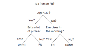
Fig 1: Decision tree example
In a Decision tree can be divided into:
● Decision Node
● Leaf Node
Decision nodes are marked by multiple branches that represent different decision
Conditions whereas output of those decisions is represented by leaf node and do not
Contain further branches.
The decision tests are performed on the basis of features of the given dataset.
It is a graphical representation for getting all the possible solutions to a problem/decision based on given conditions.
Decision Tree algorithm:
● Comes under the family of supervised learning algorithms.
● Unlike other supervised learning algorithms, decision tree algorithms can be used for solving regression and classification problems.
● Are used to create a training model that can be used to predict the class or value of the target variable by learning simple decision rules inferred from prior data (training data).
● Can be used for predicting a class label for a record we start from the root of the tree.
● Values of the root attribute are compared with the record’s attribute. On the basis of comparison, a branch corresponding to that value is considered and jumps to the next node.
Issues in Decision tree learning
● It is less appropriate for estimation tasks where the goal is to predict the value of a continuous attribute.
● This learning is prone to errors in classification problems with many classes and relatively small number of training examples.
● This learning can be computationally expensive to train. The process of growing a decision tree is computationally expensive. At each node, each candidate splitting field must be sorted before its best split can be found. In some algorithms, combinations of fields are used and a search must be made for optimal combining weights. Pruning algorithms can also be expensive since many candidate sub-trees must be formed and compared.
- Avoiding overfitting
A decision tree’s growth is specified in terms of the number of layers, or depth, it’s allowed to have. The data available to train the decision tree is split into training and testing data and then trees of various sizes are created with the help of the training data and tested on the test data. Cross-validation can also be used as part of this approach. Pruning the tree, on the other hand, involves testing the original tree against pruned versions of it. Leaf nodes are removed from the tree as long as the pruned tree performs better on the test data than the larger tree.
Two approaches to avoid overfitting in decision trees:
● Allow the tree to grow until it overfits and then prune it.
● Prevent the tree from growing too deep by stopping it before it perfectly classifies the training data.
2. Incorporating continuous valued attributes
3. Alternative measures for selecting attributes
● Prone to overfitting.
● Require some kind of measurement as to how well they are doing.
● Need to be careful with parameter tuning.
● Can create biased learned trees if some classes dominate.
Key takeaway:
● Naïve Bayes algorithm is a supervised learning algorithm, which is based on the Bayes theorem and used for solving classification problems.
● Naïve Bayes Classifier is one of the simple and most effective Classification algorithms which help in building fast machine learning models that can make quick predictions.
● Bayes’ theorem is also known as Bayes’ Rule or Bayes’ law, which is used to determine the probability of a hypothesis with prior knowledge.
● Decision Tree is a Supervised learning technique that can be used for both classification and Regression problems, but mostly it is preferred for solving Classification problems.
● It is a tree-structured classifier, where internal nodes represent the features of a dataset, branches represent the decision rules and each leaf node represents the outcome.
Scikit-learn is undoubtedly Python's most helpful machine learning library. Classification, regression, clustering, and dimensionality reduction are just a few of the useful capabilities in the sklearn toolkit for machine learning and statistical modelling.
Please keep in mind that sklearn is a tool for creating machine learning models. It should not be used for data reading, manipulation, or summarization. There are libraries that are better for that (e.g. NumPy, Pandas etc.)
Components of scikit-learn:
Scikit-learn has a lot of useful features. To help you grasp the spread, here are a few examples:
Supervised learning algorithms: Consider any supervised machine learning algorithm you've heard of, and there's a good chance it's included in scikit-learn. From generalised linear models (such as linear regression) to Support Vector Machines (SVM), Decision Trees, and Bayesian approaches, the scikit-learn toolbox has it all. One of the main reasons for scikit-popularity learn's is the widespread use of machine learning methods. I began using scikit to address supervised learning challenges, and I would recommend it to anyone who is new to scikit or machine learning.
Cross-validation: Using sklearn, you can assess the correctness of supervised models on unknown data in a variety of ways.
Unsupervised learning algorithms: The offering includes a wide range of machine learning algorithms, including clustering, factor analysis, principal component analysis, and unsupervised neural networks.
Various toy datasets: While learning scikit-learn, this came in handy. I learned SAS while working with a variety of academic datasets (e.g. IRIS dataset, Boston House prices dataset). Having them on hand while studying a new library was quite beneficial.
Feature extraction: For extracting features from photos and text, use Scikit-learn (e.g. Bag of words).
Installations
Before proceeding with the installation of Scikit-learn, we must first install a number of other tools and libraries, as we saw in the prerequisites section. So, let's start by going over how to install all of these libraries step by step, because the major goal of this tutorial is to provide information about Scikit-learn so that you can get started with it.
If any or all of these libraries are already installed, we can skip straight to the required library's installation by clicking on it:
● Installing Python
● Installing NumPy
● Installing SciPy
● Installing Scikit learn Python
For those who are unfamiliar with Python Pip (a package management system), we will also learn how to use pip to install each of these libraries individually. It's used to manage Python packages (or ones with Python dependencies).
Step 1: Installing Python
By going to the following link, we can easily install Python:
Https://www.python.org/downloads/
● Ensure that we install the most recent version, or at the very least version 2.7 or higher.
● We'll need to check if Python is available for usage on the command line after installing it. To do so, go to our system's command prompt and type 'cmd'. Type the following in the command prompt:
Python
If Python was successfully installed, it should show the Python version we're using. The Python Interpreter will be launched using this command.

Step 2: Installing NumPy
● NumPy is a basic Python module or library that allows you to conduct numerical calculations.
● Visit the following URL to download the NumPy installer, which you can then run:
Http://sourceforge.net/projects/numpy/files/NumPy/1.10.2/
● We can also install NumPy in our terminal by typing the following command:
Pip install numpy
● If we already have NumPy installed, we'll see a message that says, 'Requirement already met.'

Step 3: Installing SciPy
● SciPy is an open-source Python toolkit for doing scientific and technical computations.
● Using the following URL, download and run the SciPy installer:
Http://sourceforge.net/projects/scipy/files/scipy/0.16.1/
● By running the following command in the terminal, we can install SciPy with pip:
Pip install scipy
● If we already have SciPy, a message will appear that says, "Requirement satisfied."
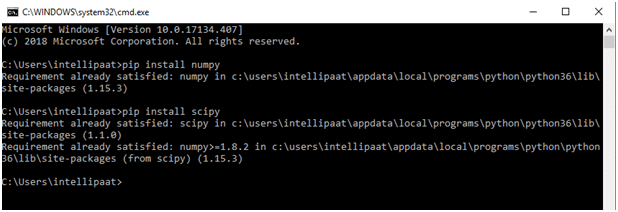
Step 4: Installing Scikit-learn
● Install Scikit-learn using pip using the following command:
Pip install Scikit-learn
● If we already have Scikit Python installed, we'll see a message that says, 'Requirement already met.'

Dataset
Toy data sets, which are basic, tidy, and occasionally fake data sets that can be used for exploratory data analysis and developing simple prediction models, are provided by Scikit-learn. Scikit-learn has some that can be used for supervised learning tasks like regression and classification.
It has a set called iris data, for example, that provides information about several varieties of iris plants. This information can be used to create, train, and test classification models that can categorise different species of iris plants based on their properties.
Loading your data is the initial step in almost any data science project. This is also where this scikit-learn tutorial begins.
This field usually deals with data that has been witnessed. You can either acquire this information yourself or look for data sets in other places. You'll probably do the latter if you're not a researcher or otherwise interested in experiments.
Finding these data sets can be difficult if you're new to this and want to start solving problems on your own. However, the UCI Machine Learning Repository and the Kaggle website are usually helpful places to look for decent data sets. Also, take a look at this KD Nuggets resource list.
For now, just load in the digits data set that comes with a Python tool called scikit-learn, and don't worry about finding any data on your own.
Mat plotlib
Matplotlib, a plotting package that can be demonstrated in Python scripts, allows for rich data plotting in an interactive manner. Plotting graphs is an element of data visualisation, and Matplotlib can help with that.
Matplotlib makes use of a variety of general-purpose GUI toolkits, including wxPython, Tkinter, QT, and others, to provide object-oriented APIs for integrating plots into applications. Matplotlib was created by John D. Hunter, and Michael Droettboom served as its principal developer. Python SciPy is a free and open-source Python library that is mostly used for technical and scientific computing. Because most scientific calculations need the plotting of graphs and diagrams, Matplotlib is commonly utilised in SciPy.
Syntax of Matplotlib Python with a Basic Example
Matplotlib is being imported. Pyplot as pltPyplot is mostly used to manipulate plots and figures.
Matplotlib.pyplot allows Python Matplotlib to function similarly to MATLAB. Let's have a look at how to use Matplotlib in Python.
Python Matplotlib Example:
Import matplotlib.pyplot as plt
Plt.plot([1,1])
Plt.plot([2,2])
Plt.plot([3,3])
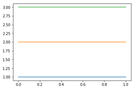
The graph can be used to plot three straight lines. We make this possible by using the plotting library, Matplotlib.
Filling missing values
Missing values are common in real-world data.
Missing values can occur for a variety of causes, including observations that were not recorded or data tampering.
Many machine learning methods do not accept data with missing values, so handling missing data is critical.
After completing this tutorial, you will be able to:
● How to indicate faulty or corrupt values in your dataset as missing.
● How to remove rows from your dataset that have missing data.
● How to fill in missing values in your dataset with mean values.
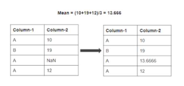
In this scenario, we'll use a certain number to fill in the blanks.
The following are some options:
● If the missing data is a numerical variable, the mean or median value is used to fill it in.
● If the missing data is a category value, use mode to fill it in.
● Filling in the numerical value with 0 or -999, or a number that will not appear in the data. This can be done in order for the system to notice that the data isn't real or isn't the same.
● For the missing values, a new type is added to the categorical value.
You can use the fillna() function to fill the null values in the dataset.
Updated_df = df
Updated_df['Age']=updated_df['Age'].fillna(updated_df['Age'].mean())
Updated_df.info()
<class 'pandas.core.frame.DataFrame'>
RangeIndex: 891 entries, 0 to 890
Data columns (total 7 columns):
# Column Non-Null Count Dtype
--- ------ -------------- -----
0 Survived 891 non-null int64
1 Pclass 891 non-null int64
2 Sex 891 non-null int64
3 Age 891 non-null float64
4 SibSp 891 non-null int64
5 Parch 891 non-null int64
6 Fare 891 non-null float64
Dtypes: float64(2), int64(5)
Memory usage: 48.9 KB
y1 = updated_df['Survived']
Updated_df.drop("Survived",axis=1,inplace=True)
From sklearn import metrics
From sklearn.model_selection import train_test_split
X_train, X_test,y_train,y_test = train_test_split(updated_df,y1,test_size=0.3)
From sklearn.linear_model import LogisticRegression
Lr = LogisticRegression()
Lr.fit(X_train,y_train)
Pred = lr.predict(X_test)
Print(metrics.accuracy_score(pred,y_test))
In this scenario, we'll use a certain number to fill in the blanks.
Python has a large number of tools for implementing classification and regression. Scikit-learn is the most popular open-source Python data science library. Let's have a look at how to utilise scikit-learn to accomplish simple classification and regression tasks.
The following are the basic steps in supervised machine learning:
● Load the necessary libraries
● Load the dataset
● Split the dataset into training and test set
● Train the model
● Evaluate the model
Loading the Libraries
#Numpy deals with large arrays and linear algebra
Import numpy as np
# Library for data manipulation and analysis
Import pandas as pd
# Metrics for Evaluation of model Accuracy and F1-score
From sklearn.metrics import f1_score,accuracy_score
#Importing the Decision Tree from scikit-learn library
From sklearn.tree import DecisionTreeClassifier
# For splitting of data into train and test set
From sklearn.model_selection import train_test_split
Loading the Dataset
Train=pd.read_csv("/input/hcirs-ctf/train.csv")
# read_csv function of pandas reads the data in CSV format
# from path given and stores in the variable named train
# the data type of train is DataFrame
Splitting into Train & Test set
#first we split our data into input and output
# y is the output and is stored in "Class" column of dataframe
# X contains the other columns and are features or input
y = train.Class
Train.drop(['Class'], axis=1, inplace=True)
X = train
# Now we split the dataset in train and test part
# here the train set is 75% and test set is 25%
X_train, X_test, y_train, y_test = train_test_split(X, y, test_size=0.25, random_state=2)
Training the model
# Training the model is as simple as this
# Use the function imported above and apply fit() on it
DT= DecisionTreeClassifier()
DT.fit(X_train,y_train)
Partitioning training and test sets
We'll create a new dataset, the Wine dataset, which may be found at https://archive.ics.uci.edu/ml/datasets/Wine in the UCI machine learning repository.
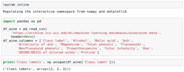
There are 178 wine samples in all, with 13 attributes for various chemical properties:


The samples are divided into three categories: 1, 2, and 3, which allude to the three different types of grapes grown in different parts of Italy.
We'll use the train test split() function from scikit-cross validation learn's submodule to randomly partition this dataset into a separate test and training dataset:


The feature columns 1-13 were assigned to the variable X, and the class labels (the first column) were assigned to the variable y, as seen in the code above.
The train test split() method was then used to split X and y into separate training and test datasets at random.
We set the test size=0.3, which indicates that 30% of the wine samples were assigned to X test and y test, while the remaining 70% were assigned to X train and y train, respectively:

Feature scaling
The process of feature scaling is used to standardise the range of features. It's also known as data normalisation (or standardisation), and it's an important stage in the data preprocessing process.
Assume we have two features, one of which is measured on a scale of 0 to 1 and the other of which is measured on a scale of 1 to 100.
Our algorithm will be largely busy managing the higher faults in the second feature while computing the squared error function or a Euclidean distance for the k-nearest neighbours (KNN).
Normalization typically refers to rescaling features in the [0, 1] range.
We may apply the min-max scaling to each feature column to normalise our data, and the new value x or m of a sample can be derived as follows:

Let's see how it's done in scikit-learn:
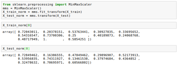
While normalisation by min-max scaling is useful for keeping values within a restricted interval, standardisation is more practical when the feature columns are expected to have a normal distribution. In contrast to min-max scaling, this makes the algorithm less susceptible to outliers:

Where and are the sample mean and standard deviation for a particular feature column, respectively.
On a sample dataset ranging from 0 to 5, the following table illustrates the differences between feature scaling, standardisation, and normalisation:
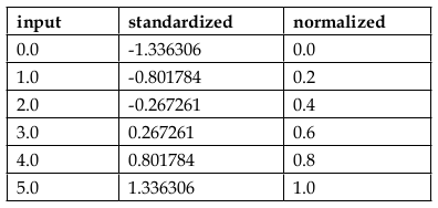
Let's look at how scikit-learn implements standardisation:

The following is a comparison of standardisation and normalisation:
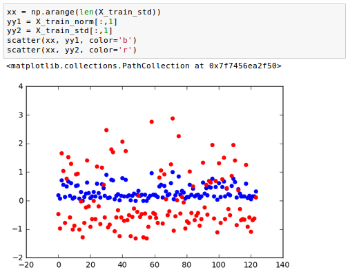
On the training data, we just used the Standard Scaler once. Then we apply the parameters we learned during training to the test set or any new data point.
References:
- Jiawei Han, Micheline Kamber, and Jian Pie, “Data Mining: Concepts and Techniques” Elsevier Publishers Third Edition, ISBN: 9780123814791, 9780123814807
- DT Editorial Services, “Big Data, Black Book”, DT Editorial Services, ISBN:
9789351197577, 2016 Edition
3. Chirag Shah, “A Hands-On Introduction To Data Science”, Cambridge University Press, (2020), ISBN : ISBN 978-1-108-47244-9