Unit – 4
Statistics and probability
Professor Bowley defines the average as-
“Statistical constants which enable us to comprehend in a single effort the significance of the whole”
An average is a single value which is the best representative for a given data set.
Measures of central tendency show the tendency of some central values around which data tend to cluster.
The following are the various measures of central tendency-
1. Arithmetic mean
2. Median
3. Mode
4. Weighted mean
5. Geometric mean
6. Harmonic mean
Arithmetic mean or mean-
Arithmetic mean is a value which is the sum of all observation divided by total number of observations of the given data set.
If there are n numbers in a dataset-  then arithmetic mean will be-

If the numbers along with frequencies are given then mean can be defined as-


Example-1: Find the mean of 26, 15, 29, 36, 35, 30, 14, 21, 25 .
Sol.


Example-2: Find the mean of the following dataset.
x | 20 | 30 | 40 |
f | 5 | 6 | 4 |
Sol.
We have the following table-
x | f | Fx |
20 | 5 | 100 |
30 | 6 | 180 |
40 | 7 | 160 |
| Sum = 15 | Sum = 440 |
Then Mean will be-


Direct method to find mean-
Example: Find the arithmetic mean of the following dataset-

Sol.
We have the following distribution-
Class interval | Mid value (x) | Frequency (f) | Fx |
0-10 | 05 | 3 | 15 |
10-20 | 15 | 5 | 75 |
20-30 | 25 | 7 | 175 |
30-40 | 35 | 9 | 315 |
40-50 | 45 | 4 | 180 |
|
| Sum = 28 | Sum = 760 |

Short cut method to find mean-
Suppose ‘a’ is assumed mean, and ‘d’ is the deviation of the variate x form a, then-

Example: Find the arithmetic mean of the following dataset.
Class | 0-10 | 10-20 | 20-30 | 30-40 | 40-50 |
Frequency | 7 | 8 | 20 | 10 | 5 |
Sol.
Let the assumed mean (a) = 25,
Class | Mid-value | Frequency | x – 25 = d | Fd |
0-10 | 5 | 7 | -20 | -140 |
10-20 | 15 | 8 | -10 | -80 |
20-30 | 25 | 20 | 0 | 0 |
30-40 | 35 | 10 | 10 | 100 |
40-50 | 45 | 5 | 20 | 100 |
Total |
| 50 |
| -20 |

Step deviation method for mean-

Where
Median-
Median is the mid value of the given data when it is arranged in ascending or descending order.
1. If the total number of values in data set is odd then median is the value of  item.
item.
Note-The data should be arranged in ascending r descending order
2. If the total number of values in data set is even then median is the mean of the  item.
item.
Example: Find the median of the data given below-
7, 8, 9, 3, 4, 10
Sol.
Arrange the data in ascending order-
3, 4, 7, 8, 9, 10
So there total 6 (even) observations, then-


=

Median for grouped data-

Here,


Example: Find the median of the following dataset-

Sol.
Class interval | Frequency | Cumulative frequency |
0 - 10 | 3 | 3 |
10 – 20 | 5 | 8 |
20 – 30 | 7 | 15 |
30 – 40 | 9 | 24 |
40 – 50 | 4 | 28 |

So that median class is 20-30.
Now putting the values in the formula-


So that the median is 28.57
Mode-
A value in the data which is most frequent is known as mode.
Example: Find the mode of the following data points-

Sol. Here 6 has the highest frequency, so that the mode is 6.
Mode for grouped data-

Here,


Example: Find the mode of the following dataset-

Sol.
Class interval | Frequency |
0 - 10 | 3 |
10 – 20 | 5 |
20 – 30 | 7 |
30 – 40 | 9 |
40 – 50 | 4 |
Here highest frequency is 9. So that the modal class is 40-50,
Put the values in the given data-


Hence the mode is 42.86
Note-
Mean – Mode = [Mean - Median]
Geometric Mean-
If  are the values of the data, then the geometric mean-

Harmonic mean-
Harmonic mean is the reciprocal of the arithmetic mean-
It can be defined as-

Note-
1. 
2. 
According to Spiegel-
“The degree to which numerical data tend to spread about an average value is called the variation or dispersion of data”
The different measures of dispersion are-
1. Range
2. Quartile deviation
3. Mean deviation
4. Standard deviation
5. Variance
Range-
This is one of the simplest measures of dispersion. The difference between the maximum and minimum value of the dataset is known as range.
Range = Max. Value – Min. Value
Example- Find the range of the data- 8, 5, 6, 4, 7, 10, 12, 15, 25, 30
Sol. Here the maximum value is 30 and minimum value is 4, so that the range is-
30 – 4 = 26
Coefficient of range-
Coefficient of range can be calculated as follows-
Coefficient of Range = 
Quartile deviation-


Example- Find the quartile deviation of the following data-
Class interval | 0-10 | 10-20 | 20-30 | 30-40 | 40-50 |
Frequency | 3 | 5 | 7 | 9 | 4 |
Sol.
Here N/4 = 28/4 = 7 so that the 7’th observation falls in the class 10 – 20.
And
3N/4 = 21, and 21’st observation falls in the interval 30 – 40 which is the third quartile.
The quartiles can be calculated as below-

And

Hence the quartile deviation is-

Mean deviation-
The mean deviation can be defined as-

Here A is assumed mean.


Example: Find the mean deviation from mean of the following data-
Class interval | 0-6 | 6-12 | 12-18 | 18-24 | 24-30 |
Frequency | 8 | 10 | 12 | 9 | 5 |
Sol.
Class interval | Mid-value | Frequency | d = x - a | f.d | |x - 14| | f |x - 14| |
0-6 | 3 | 8 | -12 | -96 | 11 | 88 |
6-12 | 9 | 10 | -6 | -60 | 5 | 50 |
12-18 | 15 | 12 | 0 | 0 | 1 | 12 |
18-24 | 21 | 9 | 6 | 54 | 7 | 63 |
24-30 | 27 | 5 | 12 | 60 | 13 | 65 |
Total |
| 44 |
| -42 |
| 278 |

Then mean deviation from mean-

Standard deviation & Variance-
Standard deviation can be defined as-

Note- The square of the standard deviation
Shortcut formula to calculate standard deviation-

The square of the standard deviation is called known as variance.

Example-1: Compute variance and standard deviation.
Class | Frequency |
0-10 | 3 |
10-20 | 5 |
20-30 | 7 |
30-40 | 9 |
40-50 | 4 |
Sol.
Class | Mid-value (x) | Frequency (f) |  |
0-10 | 5 | 3 | 1470.924 |
10-20 | 15 | 5 | 737.250 |
20-30 | 25 | 7 | 32.1441 |
30-40 | 35 | 9 | 555.606 |
40-50 | 45 | 4 | 1275.504 |
Sum |
|  | 4071.428 |

Then standard deviation,

Example-2: Calculate the standard deviation of the following frequency distribution-
Weight | 60 – 62 | 63 – 65 | 66 – 68 | 69 – 71 | 72 – 74 |
Item | 5 | 18 | 42 | 27 | 8 |
Sol.
Weight | Item (f) | x | d = x – 67 | f.d |  |
60 – 62 | 5 | 61 | -6 | -30 | 180 |
63 – 65 | 18 | 64 | -3 | -54 | 162 |
66 – 68 | 42 | 67 | 0 | 0 | 0 |
69 – 71 | 27 | 70 | 3 | 81 | 243 |
72 – 74 | 8 | 73 | 6 | 48 | 288 |
Total |
100 |
|
|
45 |
873 |


Coefficient of variation can be calculated as-

Note- The lower value of C.V, the more constancy of data
Example- If a student A has mean 50 with SD 10.Another student B has mean 30 with SD = 3.
Which one is the best performer?
Sol. We calculate C.V.-


And

Here B has lower C.V., so that student B is the best performer.
Moments-
The r’th moment of a variable x about the mean is denoted by  and defined as-

The r’th moment of a variable x about any point ‘a’ will be-

Relationship between moments about mean and moment about any point-

Skewness-
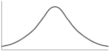
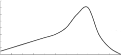
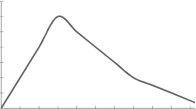
The word skewness means lack of symmetry-
The examples of symmetric curve, positively skewd and negatively skewd curves are given as follows-
1. Symmetric curve-
2. Positively skewd-
3. Negatively skewd-
To measure the skewness we use Karl Pearson’s coefficient of skewness.
Then formula is as follows-

Note- the value of Karl Pearson’s coefficient of skewness lies between -1 to +1.
Kurtosis-
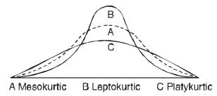
It is the measurement of the degree of peakedess of a distribution
Kurtosis is measured as-
Calculation of kurtosis-
The second and fourth central moments are used to measure kurtosis.
We use Karl Pearson’s formula to calculate kurtosis-

Now, three conditions arises-
1. If  , then the curve is mesokurtic.
2. If  , then the curve is platykurtic
3. If  , then the curve is said to be leptokurtic.
Example: If coefficient of skewness is 0.64. Standard deviation is 13 and mean is 59.2, then find the mode and median.
Sol.
We know that-

So that-


And we also know that-


Example: Calculate the Karl Pearson’s coefficient of skewness of marks obtained by 150 students.

Sol. Mode is not well defined so that first we calculate mean and median-
Class | f | x | CF |  | Fd |  |
0-10 | 10 | 5 | 10 | -3 | -30 | 90 |
10-20 | 40 | 15 | 50 | -2 | -80 | 160 |
20-30 | 20 | 25 | 70 | -1 | -20 | 20 |
30-40 | 0 | 35 | 70 | 0 | 0 | 0 |
40-50 | 10 | 45 | 80 | 1 | 10 | 10 |
50-60 | 40 | 55 | 120 | 2 | 80 | 160 |
60-70 | 16 | 65 | 136 | 3 | 48 | 144 |
70-80 | 14 | 75 | 150 | 4 | 56 | 244 |
Now,


And

Standard deviation-

Then-


When two variables are related in such a way that change in the value of one variable affects the value of the other variable, then these two variables are said to be correlated and there is correlation between two variables.
Example- Height and weight of the persons of a group.
The correlation is said to be perfect correlation if two variables vary in such a way that their ratio is constant always.
Scatter diagram-
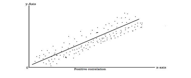
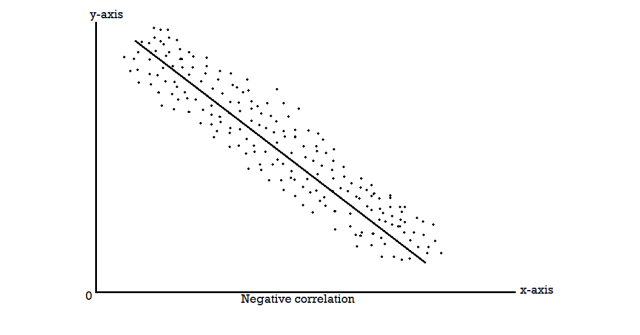
Karl Pearson’s coefficient of correlation-

Here-  and
and 

Note-
1. Correlation coefficient always lies between -1 and +1.
2. Correlation coefficient is independent of change of origin and scale.
3. If the two variables are independent then correlation coefficient between them is zero.
Correlation coefficient | Type of correlation |
+1 | Perfect positive correlation |
-1 | Perfect negative correlation |
0.25 | Weak positive correlation |
0.75 | Strong positive correlation |
-0.25 | Weak negative correlation |
-0.75 | Strong negative correlation |
0 | No correlation |
Example: Find the correlation coefficient between Age and weight of the following data-
Age | 30 | 44 | 45 | 43 | 34 | 44 |
Weight | 56 | 55 | 60 | 64 | 62 | 63 |
Sol.
x | y |  |  |  |  | (   |
30 | 56 | -10 | 100 | -4 | 16 | 40 |
44 | 55 | 4 | 16 | -5 | 25 | -20 |
45 | 60 | 5 | 25 | 0 | 0 | 0 |
43 | 64 | 3 | 9 | 4 | 16 | 12 |
34 | 62 | -6 | 36 | 2 | 4 | -12 |
44 | 63 | 4 | 16 | 3 | 9 | 12 |
Sum= 240 |
360 |
0 |
202 |
0 |
70
|
32 |
Karl Pearson’s coefficient of correlation-

Here the correlation coefficient is 0.27.which is the positive correlation (weak positive correlation), this indicates that the as age increases, the weight also increase.
Short-cut method to calculate correlation coefficient-

Here,


Example: Find the correlation coefficient between the values X and Y of the dataset given below by using short-cut method-
X | 10 | 20 | 30 | 40 | 50 |
Y | 90 | 85 | 80 | 60 | 45 |
Sol.
X | Y |  |  |  |  |  |
10 | 90 | -20 | 400 | 20 | 400 | -400 |
20 | 85 | -10 | 100 | 15 | 225 | -150 |
30 | 80 | 0 | 0 | 10 | 100 | 0 |
40 | 60 | 10 | 100 | -10 | 100 | -100 |
50 | 45 | 20 | 400 | -25 | 625 | -500 |
Sum = 150 |
360 |
0 |
1000 |
10 |
1450 |
-1150 |
Short-cut method to calculate correlation coefficient-


Spearman’s rank correlation-
When the ranks are given instead of the scores, then we use Spearman’s rank correlation to find out the correlation between the variables.
Spearman’s rank correlation coefficient can be defined as-

Example: Compute the Spearman’s rank correlation coefficient of the dataset given below-
Person | A | B | C | D | E | F | G | H | I | J |
Rank in test-1 | 9 | 10 | 6 | 5 | 7 | 2 | 4 | 8 | 1 | 3 |
Rank in test-2 | 1 | 2 | 3 | 4 | 5 | 6 | 7 | 8 | 9 | 10 |
Sol.
Person | Rank in test-1 | Rank in test-2 | d =  |  |
A | 9 | 1 | 8 | 64 |
B | 10 | 2 | 8 | 64 |
C | 6 | 3 | 3 | 9 |
D | 5 | 4 | 1 | 1 |
E | 7 | 5 | 2 | 4 |
F | 2 | 6 | -4 | 16 |
G | 4 | 7 | -3 | 9 |
H | 8 | 8 | 0 | 0 |
I | 1 | 9 | -8 | 64 |
J | 3 | 10 | -7 | 49 |
Sum |
|
|
| 280 |


Regression-
Regression is the measure of average relationship between independent and dependent variable
Regression can be used for two or more than two variables.
There are two types of variables in regression analysis.
1. Independent variable
2. Dependent variable
The variable which is used for prediction is called independent variable.
It is known as predictor or regressor.
The variable whose value is predicted by independent variable is called dependent variable or regressed or explained variable.
The scatter diagram shows relationship between independent and dependent variable, then the scatter diagram will be more or less concentrated round a curve, which is called the curve of regression.
When we find the curve as a straight line then it is known as line of regression and the regression is called linear regression.
Note- regression line is the best fit line which expresses the average relation between variables.
Equation of the line of regression-
Let
y = a + bx ………….. (1)
Is the equation of the line of y on x.
Let  be the estimated value of
  for the given value of
  .
.
So that, According to the principle of least squares, we have the determined ‘a’ and ‘b’ so that the sum of squares of deviations of observed values of y from expected values of y,
That means-

Or
 …….. (2)
Is minimum.
Form the concept of maxima and minima, we partially differentiate U with respect to ‘a’ and ‘b’ and equate to zero.
Which means


And


These equations (3) and (4) are known as normal equation for straight line.
Now divide equation (3) by n, we get-

This indicates that the regression line of y on x passes through the point .
.
We know that-

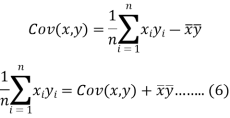
The variance of variable x can be expressed as-


Dividing equation (4) by n, we get-

From the equation (6), (7) and (8)-

Multiply (5) by , we get-

Subtracting equation (10) from equation (9), we get-


Since ‘b’ is the slope of the line of regression y on x and the line of regression passes through the point ( ), so that the equation of the line of regression of y on x is-


This is known as regression line of y on x.
Note-
 are the coefficients of regression.
2. 
Example: Two variables X and Y are given in the dataset below, find the two lines of regression.
x | 65 | 66 | 67 | 67 | 68 | 69 | 70 | 71 |
y | 66 | 68 | 65 | 69 | 74 | 73 | 72 | 70 |
Sol.
The two lines of regression can be expressed as-

And

x | y |  |  | Xy |
65 | 66 | 4225 | 4356 | 4290 |
66 | 68 | 4356 | 4624 | 4488 |
67 | 65 | 4489 | 4225 | 4355 |
67 | 69 | 4489 | 4761 | 4623 |
68 | 74 | 4624 | 5476 | 5032 |
69 | 73 | 4761 | 5329 | 5037 |
70 | 72 | 4900 | 5184 | 5040 |
71 | 70 | 5041 | 4900 | 4970 |
Sum = 543 | 557 | 36885 | 38855 | 37835 |
Now-

And

Standard deviation of x-


Similarly-


Correlation coefficient-


Put these values in regression line equation, we get
Regression line y on x-


Regression line x on y-


Regression line can also be find by the following method-
Example: Find the regression line of y on x for the given dataset.
X | 4.3 | 4.5 | 5.9 | 5.6 | 6.1 | 5.2 | 3.8 | 2.1 |
Y | 12.6 | 12.1 | 11.6 | 11.8 | 11.4 | 11.8 | 13.2 | 14.1 |
Sol.
Let y = a + bx is the line of regression of y on x, where ‘a’ and ‘b’ are given as-


We will make the following table-
x | y | Xy |  |
4.3 | 12.6 | 54.18 | 18.49 |
4.5 | 12.1 | 54.45 | 20.25 |
5.9 | 11.6 | 68.44 | 34.81 |
5.6 | 11.8 | 66.08 | 31.36 |
6.1 | 11.4 | 69.54 | 37.21 |
5.2 | 11.8 | 61.36 | 27.04 |
3.8 | 13.2 | 50.16 | 14.44 |
2.1 | 14.1 | 29.61 | 4.41 |
Sum = 37.5 | 98.6 | 453.82 | 188.01 |
Using the above equations we get-


On solving these both equations, we get-
a = 15.49 and b = -0.675
So that the regression line is –
y = 15.49 – 0.675x
Note – Standard error of predictions can be find by the formula given below-

Difference between regression and correlation-
1. Correlation is the linear relationship between two variables while regression is the average relationship between two or more variables.
2. There are only limited applications of correlation as it gives the strength of linear relationship while the regression is to predict the value of the dependent varibale for the given values of independent variables.
3. Correlation does not consider dependent and independent variables while regression consider one dependent variable and other indpendent variables.
Probability is the study of chances. Probability is the measurement of the degree of uncertainty and therefore, of certainty of the occurrence of events.
Some important definitions-
Random experiment-
An experiment in which all the possible outcomes are known in advance but we cannot predict as to which of them will occur when we perform the experiment.
Example-‘Throwing a die’ and ‘Drawing a card from a well shuffled pack of 52 playing cards ‘are the examples of random experiment
Sample space-
Set of all possible outcomes of a random experiment is known as sample space and is usually denoted by S.
Example-
1. If we toss a coin then the sample space is
S = {H, T}, where H and T denote head and tail respectively and n(S) = 2
2. If a coin is tossed thrice or three coins are tossed simultaneously, then the sample space is
S = {HHH, HHT, HTH, THH, HTT, THT, TTH, TTT} and n(S) = 8.
3. If a coin is tossed 4 times or four coins are tossed simultaneously then the sample space is
S = {HHHH, HHHT, HHTH, HTHH, THHH, HHTT, HTHT, HTTH, THHT,
THTH, TTHH, HTTT, THTT, TTHT, TTTH, TTTT} and n(S) = 16.
Sample point-
Each outcome of an experiment is visualised as a sample point in the sample space.
Example- If a die is thrown twice, then getting (1, 1) or (1, 2) or (1, 3) or…or (6, 6) is a sample point.
Event-
Set of one or more possible outcomes of an experiment constitutes what is known as event. Thus, an event can be defined as a subset of the sample space
Exhaustive cases-
The total number of possible outcomes in a random experiment is called the exhaustive cases
Example-If we throw a die then number of exhaustive cases is 6 and the sample space in this case is {1, 2, 3, 4, 5, 6}
Favourable cases-
The cases which favour to the happening of an event are called favourable cases
Example-For the event of getting an even number in throwing a die, the number of favourable cases is 3 and the event in this case is {2, 4, 6}.
Mutually exclusive cases-
Cases are said to be mutually exclusive if the happening of any one of them prevents the happening of all others in a single experiment
Equally likely cases-
Two events are said to be ‘equally likely’, if one of them cannot be expected in preference to the other.
Example-if we draw a card from well-shuffled pack, we may get any card, then the 52 different cases are equally likely.
Odds in favour of an event and odds against an event-
If the number of favourable cases are ‘m’ and the number or not favourable cases are ‘n’.
Then-
1. Odds in favour of the event = m/n
2. Odds against the event = n/m
Classical definition of probability-
Suppose there are ‘n’ exhaustive cases in a random experiment which is equally likely and mutually exclusive.
Let ‘m’ cases are favourable for the happening of an event A, then the probability of happening event A can be defined as-

Probability of non-happening of the event A is defined as-

Note- Always remember that the probability of any events lies between 0 and 1.

Expected value-
Let  are the probabilities of events and
  respectively. Then the expected value can be defined as-

Example: A bag contains 7 red and 8 black balls then find the probability of getting a red ball.
Sol.
Here total cases = 7 + 8 = 15
According to the definition of probability,

So that, here favourable cases- red balls = 7
Then,

Addition and multiplication law of probability-
Addition law-
If  are the probabilities of mutually exclusive events, then the probability P, that any of these events will happen is given by
Note-
If two events A and B are not mutually exclusive then then probability of the event that either A or B or both will happen is given by-

Example: A box contains 4 white and 2 black balls and a second box contains three balls of each colour. Now a bag is selected at random and a ball is drawn randomly from the chosen box. Then what will be the probability that the ball is white.
Sol.
Here we have two mutually exclusive cases-
1. The first bag is chosen
2. The second bag is chosen
The chance of choosing the first bag is 1/2. And if this bag is chosen then the probability of drawing a white ball is 4/6.
So that the probability of drawing a white ball from first bag is-

And the probability of drawing a white ball from second bag is-

Here the events are mutually exclusive, then the required probability is-


Example-25 lottery tickets are marked with first 25 numerals. A ticket is drawn at random.
Find the probability that it is a multiple of 5 or 7.
Sol:
Let A be the event that the drawn ticket bears a number multiple of 5 and B be the event that it bears a number multiple of 7.
So that
A = {5, 10, 15, 20, 25}
B = {7, 14, 21}
Here, as A  B =
B =  ,
,
A and B are mutually exclusive
Then,

Multiplication law-
For two events A and B-


Here  is called conditional probability of B given that A has already happened.
Now-
If A and B are two independent events, then-

Because in case of independent events- 
Example: A bag contains 9 balls, two of which are red three blue and four black.
Three balls are drawn randomly. What is the probability that-
1. The three balls are of different colours
2. The three balls are of the same colours.
Sol.
1. Three balls will be of different colour if one ball is red, one blue and one black ball are drawn-
Then the probability will be-

2. Three balls will be of same colour if one ball is red, one blue and one black ball are drawn-
Then the probability will be-

Example: A die is rolled. If the outcome is a number greater than three. What is the probability that it is a prime number.
Sol.
The sample space is- S = {1, 2, 3, 4, 5, 6}
Let A be the event that the outcome is a number which is greater than three and B be the event that it is a prime.
So that-
A = {4, 5, 6} and B = {2, 3, 5} and hence 
P(A) = 3/6, P(B) = 3/6 and 
Now the required probability-


Example: Two cards are drawn from a pack of playing cards in succession with replacement of first card. Find the probability that the both are the cards of heart.
Sol.
Let A be the event that first card drawn is a heart and B be the event that second card is a heart card.
As the cards are drawn with replacement,
Here A and B are independent and the required probability will be-

Example: Two male and female candidates appear in an interview for two positions in the same post. The probability that the male candidate is selected is 1/7 and the female candidate selected is 1/5.
What is the probability that-
1. Both of them will be selected
2. Only one of them will be selected
3. None of them will be selected.
Sol.
Here, P (male’s selection) = 1/7
And
P (female’s selection) = 1/5
Then-
1.

2.


3.

Example: A can hit a target 3 times in 5 shots, B 2 times in 5 shots and C 3 times in 4 shots. All of them fire one shot each simultaneously at the target.
What is the probability that-
1. Two shots hit
2. At least two shots hit
Sol.


1. Now probability that 2 shots hit the target-


2.
Probability of at least two shots hitting the target


Conditional Probability-
Suppose A and B are two events of a sample space S and P(B) is non-zero, then conditional probability of the event A, given B,
It is given by P(A/B) and read as Probability of A given B-
Defined by-


Bayes theorem-
Let S be a sample space and  be n mutually exclusive events with P(
 .
.
Let A be any event which is a sub-set of  with P(A)>0, then-
 =
= 
Where i = 1, 2, ……. ,n
And  [which is law of total probability]
Example- Three urn contains 6 red, 4 black; 4 red, 6 black; 5 red, 5 black balls respectively. One of the urn is selected randomly and a ball drawn from it.
If the ball drawn is red then find the probability that it is drawn from the first urn.
Sol.
Let,


Now we have to find- 
By using Bayes theorem-
 =
= 
Here three urns equally likely to be selected-
So that-

And-


So that-
 =
= 
Hence the required probability is 2/5.
Example: A person speaks truth 3 out of 4 times. A die is thrown. She reports that there is five. What is the chance there is 5.
Sol.
Let  be the event that the person speak truth,
  be the event that she tells lie and A be the event that she reports a five.
So that-
By the law of total probability-


Now we have to find- 
By using Bayes theorem-
 =
= 
 =
= 
Which is the required probability.
Probability density function-
Let f(x) be a continuous function of x, then-

Is called probability density function.
Note- if X is a continuous random variable and  then-
then-


Where-
1. 
2. 
The set of values  with their probabilities
  constitute a discrete probability distribution of the discrete variable X.
Binomial distribution-
A discrete random variable X is said to be follow the binomial distribution with parameter n and p.
The probability of happening of an event r times exactly in n trials is-

Example: A die is thrown 8 times then find the probability that 3 will show-
1. Exactly 2 times
2. At least 7 times
3. At least once
Sol.
As we know that-


Then-
1. Probability of getting 3 exactly 2 times will be-

2. Probability of getting 3 at least 7 or 8 times will be-

3. Probability of getting 3 at least once or (1 or 2 or 3 or 4 or 5 or 6 or 7 or 8 times)-


Example: If the percentage of failure in a test is 20. If six students appear in the test, then what will be the probability that at least five students will pass the test?
Sol.
Here


Then the probability of at least five students will pass the test-


Mean and standard deviation of binomial distribution-
1. 
2. 
3. 
Moments of binomial distribution-
1. First moment about the origin-

2. Second moment about the origin-

3. Third moment about origin-

4. Fourth moment about origin-

5. Third central moment-

6. Fourth central moment-

Example: Find mean and variance of a binomial distribution with p = 1/4 and n = 10.
Sol.
Here 
Mean = np = 
Variance = npq = 
Example: If a dice is rolled thrice. A success is getting 1 or 6 on a roll. Find the mean variance of the number of success.
Sol.
Here n = 3 , p = 1/3 and q = 2/3
Mean = np = 1
And variance = npq = 2/3
Poisson distribution-
Poisson distribution is a limiting case of binomial distribution under certain conditions listed below-
1. n, the number of trials are infinitely large.
2. p, the probability of success for each trial is very small.
3. Np is finite quantity say 
A random variable X is said to be follow Poisson distribution if it has the following probability mass function-


Moments of Poisson distribution-
1. First moment about origin-  which Is known as mean.
2. Second moment about origin- 
3. Third moment about origin- 
4. Fourth moment about origin- 
Note-
1. Poisson distribution is always positively skewed distribution.
2. Mean and variance of Poisson dist. Are always equal
For Poisson distribution-


Example: If cars arriving at workshop follow the Poisson distribution. If the average number of cars arrivals during a specified period of an hour is 2.
Find the probabilities that during the given hour-
1. No car arrive
2. At least two cars arrive.
Sol.
Here the average of car arrivals is - 2
So that mean = 2

Let X be the number of cars arriving during the given hour,
By using Poisson distribution, we get-

So that the required probability-
1. P [no car will arrive] = P [X = x] = 
2. P [At least two cars will arrive] = P [X≥2] = P [X =2] + P [X = 3] + ……….
= 1 - P [[X =1] + P [X =0]]


Example: If the probability that a vaccine given to the patients shows bad reaction is 0.001, then find the probability that out of 2000 patients-
1. Exactly 3 patients
2. More than 2 patients
3. No patient
Will show bad reaction.
Sol.
Here p = 0.001 and number of patients (n) = 2000
Then 
By using Poisson distribution, we get-

1. Probability that exactly 3 patients show bad reaction is-

2. Probability that more than 2 patients show bad reaction-


3. Probability that no patient shows bad reaction-

Example: If a book has 600 pages and it has 40 printing mistakes. Assume that these mistakes are randomly distributed and x the number of mistakes per page follow Poisson distribution.
What is the probability that there will not be any mistake if 10 pages selected at random?
Sol.
Here 
We get by using Poisson distribytion-

Then-

Normal Distribution-
The concept of normal distribution was given by English mathematician Abraham De Moivre in 1733 but the concrete theory was given by Karl Gauss that is why sometime normal distribution is called Gaussian distribution.
Normal distribution is a continuous distribution. It is a limiting case of binomial distribution.
The probability density function of a normal distribution is given by-

Here 
Where 
Note-
1. If a random variable X follows normal distribution with mean  and variance
  then we can write it as- X
2. If X  , then
  is called standard normal variate with mean 0 and standard deviation 1.
3. The probability density function of standard normal variate Z is given as-

Where 
Graph of a normal probability function-
The curve look like bell-shaped curve. The top of the bell is exactly above the mean.
If the value of standard deviation is large then curve tends to flatten out and for small standard deviation it has sharp peak.
This is one of the most important probability distributions in statistical analysis.
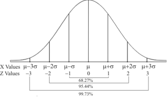
Example:
1. If X  then find the probability density function of X.
2. If X  then find the probability density function of X.
Sol.
1. We are given X 
Here 
We know that-

Then the p.d.f. will be-

2. . We are given X 
Here 
We know that-

Then the p.d.f. will be-

Mean, median and mode of the normal distribution-
Let ‘a’ is the median, then it divides the total area into two parts-

Where-

Let a>mean, then-
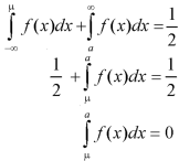
Thus-

So that mean = median.
Note- mean deviation about mean is = 
Mode-
The mode of the normal distribution is  and modal ordinate is given by-

Hence the mean, median and mode are equal in normal distribution.
Area property of a normal distribution (Area under the normal curve)-
Let X follows the normal distribution with mean  and variance
We form a normal curve by taking 
Note- Total area under the curve is always 1.
Example: If a random variable X is normally distributed with mean 80 and standard deviation 5, then find-
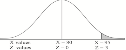
1. P[X > 95]
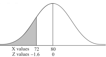
2. P[X < 72]
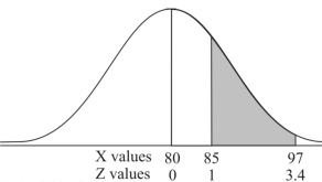
3. P [85 < X <97]
[Note- use the table- area under the normal curve]
Sol.
The standard normal variate is – 
Now-
1. X = 95,

So that-


2. X = 72,

So that-


3. X = 85,

X = 97,

So that-


Example: In a company the mean weight of 1000 employees is 60kg and standard deviation is 16kg.
Find the number of employees having their weights-
1. Less than 55kg.
2. More than 70kg.
3. Between 45kg and 65kg.
Sol. Suppose X be a normal variate = the weight of employees.
Here mean 60kg and S.D. = 16kg
X 
Then we know that-

We get from the data,

Now-
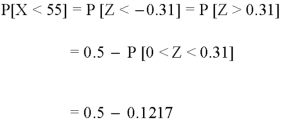
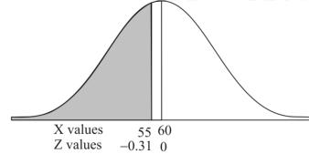
1. For X = 55,

So that-

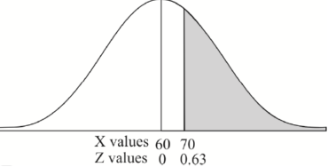
2. For X = 70,

So that-


3. For X = 45,

For X = 65,


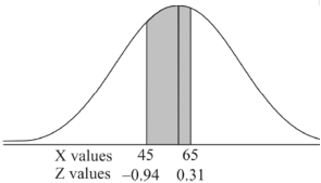
Hence the number of employees having weights between 45kg and 65kg-

Example: The mean inside diameter of a sample of 200 washers produced by a machine is 0.0502 cm and the standard deviation is 0.005 cm. The purpose for which these washers are intended allows a maximum tolerance in the diameter of 0.496 to 0.508 cm, otherwise the washers are considered defective. Determine the percentage of defective washers produced by the machine, assuming the diameters are normally distributed.
Sol.
Here-

And

Area for non-defective washers = area between z = -1.2 to +1.2
= 2 area between z = 0 and z = 1.2
= 2 × 0.3849 = 0.7698 = 76.98%
Then percent of defective washers = 100 – 76.98 = 23.02 %
Example: The life of electric bulbs is normally distributed with mean 8 months and standard deviation 2 months.
If 5000 electric bulbs are issued how many bulbs should be expected to need replacement after 12 months?
[Given that P (z ≥ 2) = 0. 0228]
Sol.
Here mean (μ) = 8 and standard deviation = 2
Number of bulbs = 5000
Total months (X) = 12
We know that-

Area (z ≥ 2) = 0.0228
Number of electric bulbs whose life is more than 12 months ( Z > 12)
= 5000 × 0.0228 = 114
Therefore replacement after 12 months = 5000 – 114 = 4886 electric bulbs.
Test of hypothesis-
Based on the given information, we draw certain conclusion about the population.
These conclusion made by some assumptions. These assumptions are called statistical hypothesis.
Null hypothesis-
The hypothesis which we test is known as the null hypothesis.
R.A. Fisher defined null hypothesis as-
“A null hypothesis is a hypothesis which is tested for possible rejection under the assumption that it is true”
The hypothesis against the null hypothesis is called alternative hypothesis ( .
.
The null hypothesis is denoted by 
Two types of errors-
Decision |  |  |
 |  |  |
 |  |  |
Type-I error-
If we reject the null hypothesis  when it is true is called type-I error. The probability of type-I error is called size of test, and it is denoted by α.
Type-II error-
If we do not reject the null hypothesis  when it is false is called type-I error.
The probability of type-I error is denoted by β.
(1 – β) is the probability of correct decisions and it is known as the power of the test.
Level of significance-
The probability of type-I error is known as level of significance of a test. It is also called the critical region and denoted by α.
It is pre-fixed as 5% or 1% level of significance.
Note- the probability of the value of the variate falling in the critical region is the level of significance. If it falls in the critical region then the hypothesis is rejected.
One tailed and two tailed tests-
A test of testing the null hypothesis is said to be two-tailed test if the alternative hypothesis is two-tailed whereas if the alternative hypothesis is one-tailed then a test of testing the null hypothesis is said to be one-tailed test.

Confidence limits-
The 95% confidence limits are  .
.
If a sample statistic lies between the intervals then we call it 95% confidence interval.
If a sample statistic lies between the intervals then we call it 99% confidence interval.
The numbers 1.96 and 2.58 are the confidence coefficients.
Test of significance of large samples-
For normal distribution 5% of the observations lie outside  and only 1% lie outside
Note- Normal distribution is the limiting case of binomial distribution when the data points are large.

Here z is the standard normal variate.
We find the value of z.
Now test of significance based on the value of z-
1. If |z|<1.96, difference between the observed and expected number of successes is not significant at the 5% level of significance.
2. If |z|>1.96, difference is significant at the 5% level of significance.
3. If |z|<2.58, difference between the observed and expected number of successes is not significant at the 1% level of significance.
4. If |z|>2.58, difference is significant at the 1% level of significance.
Formation of hypotheses-
Example: A company has replaced its original technology of producing electric bulbs by CFL technology. The company manager wants to compare the average life of bulbs manufactured by original technology and new technology CFL. Write appropriate null and alternate hypotheses
Sol.
Let the average life of original and CFL technology bulbs are denoted by  and
and  .
.
The null and alternative hypotheses will be-


Here the alternate hypothesis is two tailed so that the test will also be two tailed.
If the manager is interested just to know whether average life of CFL is greater than the original technology bulbs then the null and alternative hypotheses will be-


Here the alternative hypothesis is left tailed so that the corresponding test will also be left tailed.
Step by step method of testing a hypothesis-
Step-1 first setup the null and alternative hypothesis. Let we want to test the assumed value of  of parameter
  .
.
We can take the null and alternative hypothesis as-


Or


In case of two populations-


Or


Step-2: Establish a criteria for rejection or non-rejection of null hypothesis, that is decide the level of significance at which we want to test our hypothesis. Generally we take it as 5% or 1% level of significance.
Step-3: Now choose the appropriate test statistic under  for testing the null hypothesis.

And that specify the sampling distribution of the test statistic in the standard form Z, chi-square, t and F.
Step-4: Calculate the value of test statistic as in step-3 on the basis of observed sample observations.
Step-5: Get the critical value in the sampling distribution of the test statistic and make rejection region of α.
Step-6: Now compare the calculated value of test statistic with the critical value and find that it lies in rejection or non-rejection region
Step-7: Now we come across two situations-
1. If the calculated value of test statistic lies in rejection region at the level of significance then we reject the null hypothesis.
That means the sample data provides us significant decision against the null hypothesis.
2. If calculated value of test statistic lies in non-rejection region at level of significance then we do not reject null hypothesis. Its means that the sample data fails to provide us sufficient evidence against the null hypothesis.
Example: A manufacturer of electric bulbs claims that a certain pen manufactured by him has a mean life at least 460 days. An purchasing officer selects a sample of 100 bulbs and put them on the test. The mean life of the sample found 453 days with standard deviation 25 days. Should the purchasing officer reject the manufacturer’s claim at 1% level of significance?
Sol.
Here the population mean = 
Sample size = n = 100
Sample mean = 
Sample standard deviation = S = 25
The null and alternative hypotheses will be-

Here alternative hypothesis is left tailed so that the test is left tailed test-
Here population standard deviation is unknown so that we should use t-test if life of the bulbs follows normal distribution.
But it is not the case. Here sample size is 100 which is large.
Note- sample size more than 30 is considered as large sample.
So here we use Z-test-


Critical value of Z statistic at 1% level of significance is = -2.33
Since the calculated value of test statistic is less than the critical value that means test statistic lies in rejection region.
Therefore we reject the null hypothesis.
So that we reject the manufacturer’s claim at 1% level of significance.
Chi-square test-
The chi-square test works under the following circumstances-
1. When the given data is normally distributed.
2. Sample observations are random and independent.
Let  be a random sample of size n taken from a normal population with mean
  and variance
  . Where mean and variance are not known.
General procedure of chi-square test-
We want to test the claim about the specified value  of population variance
  then-
then-
For testing the null and alternative hypotheses, the test statistic is defined as-

Here

Here the test statistic follows chi-square distribution with (n-1) degrees of freedom.
Example: The12 measurements of the same object on an instrument are given below-
1.6, 1.5, 1.3, 1.5, 1.7, 1.6, 1.5, 1.4, 1.6, 1.3, 1.5, 1.5
If the measurement of the instrument follows normal distribution then carry out the test at 1% level of significance that variance in the measurement of the instrument is less than 0.016.
Sol.
Here the sample size = n = 12
Specified value of population variance under test = 
Here we want to test that the variance is the measurement of the instrument is less than 0.016.
The null and alternative hypotheses are-

Here the alternative hypothesis is left tailed then the test is also left tailed test.
Sample size is small and the measurement of the instruments follows normal distribution so that we will use chi-square test for population variance.
The test statistic of chi-square test is defined as-

X |  |  |
1.6 | 0.1 | 0.01 |
1.5 | 0 | 0 |
1.3 | -0.2 | 0.04 |
1.5 | 0 | 0 |
1.7 | 0.2 | 0.04 |
1.6 | 0.1 | 0.01 |
1.5 | 0 | 0 |
1.4 | -0.1 | 0.01 |
1.6 | 0.1 | 0.01 |
1.3 | -0.2 | 0.04 |
1.5 | 0 | 0 |
1.5 | 0 | 0 |
Sum = 18 | 0 | 0.16 |
From the table-
Mean= 18/12 = 1.5
And

The critical value of the test statistic at 5% level of significance is = 4.57.
Here the calculated value of test statistic is greater than the critical value.
That means the value of test statistic lies in non-rejection region so that we do not reject the null hypothesis. Hence we reject the claim at 5% level of significance
We conclude that the variance in the measurement of the instruments is not less than 0.016.