Unit-4
Laplace Transform
It is a technique for solving differential equations. The time-domain differential equations are transformed into the algebraic equation of the frequency domain. After solving the algebraic equation in the frequency domain, the result then is finally transformed to time domain form to achieve the ultimate solution of the differential equation.
The Laplace Transform is given as
F(s)= dt
dt
The advantages of Laplace Transform are:
1) It is systematic.
2) It gives a total solution (transient and sustained solution) in one operation.
3) The initial conditions are automatically specified in the transformed equations.
Key takeaway
Many functions do not have Laplace Transforms. These functions are not generally used in the analysis of linear systems. But some conditions can be defined to get Laplace transformation of such functions. The Dirichlet condition defines the necessary condition for the transformation of some functions such as:
a) The function should be continuous. The function should be single-valued.
b) The function must be of exponential order.
Properties of Laplace Transform:
1) Linearity Property:
If f1(t) and f2(t) are two functions of time. Then, in the domain of convergence
L[a f1(t)+b f2(t)]=a + b
+ b
=aF1(s)+bF2(s)
2) Differentiation Property:
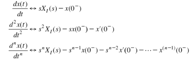
If x(t) is a function of time then Laplace transform of the nth derivative is given as
3) Integration Property:
The Laplace of nth order integral is given as
L[ ]=
]= +
+
L[f-n(t)]= +
+ +
+ +……….
+……….
As 
 ……..=0. Hence
L[f-n(t)]=
Key takeaway
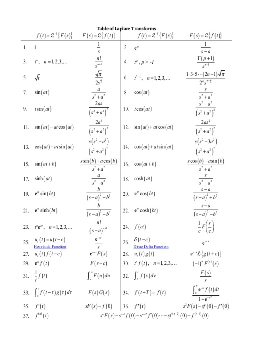
Laplace Transform of some common functions
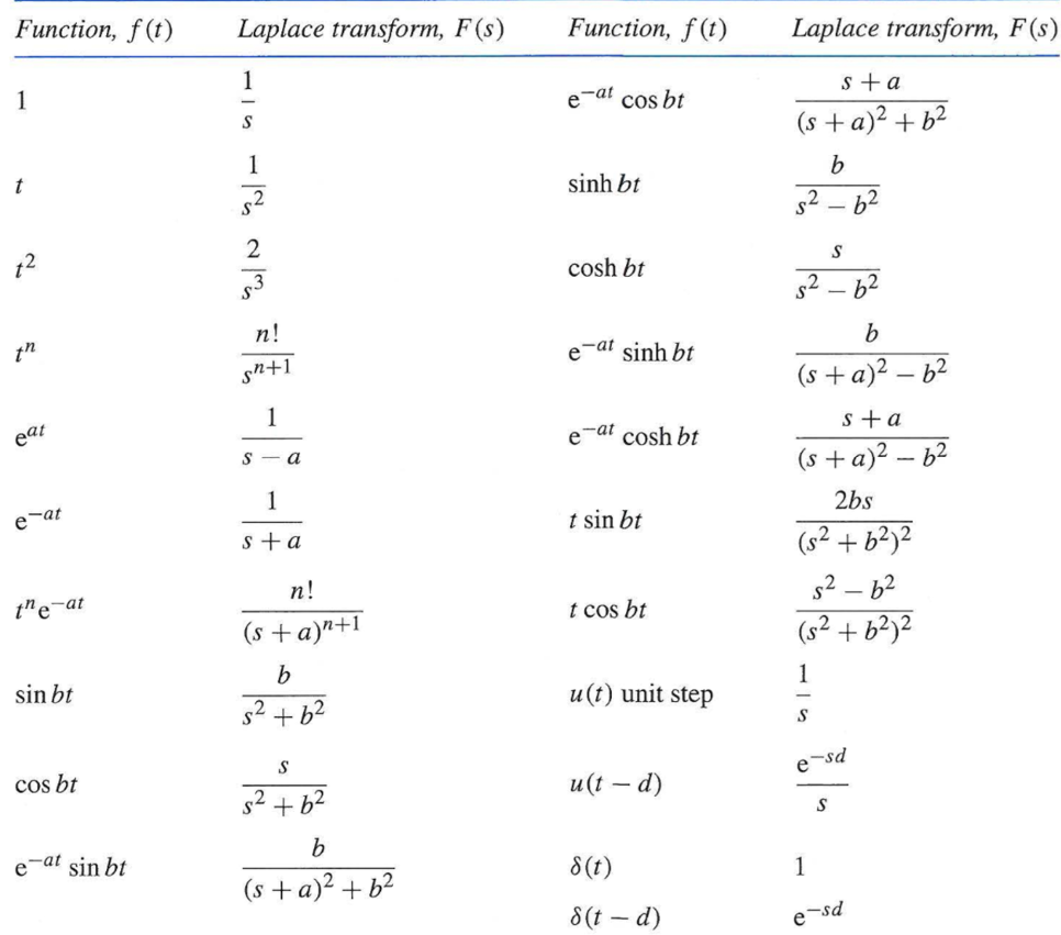
LAPALACE TRANSFORM:
If LT[f(t)]= F(s)
Where F(s)= dt
dt
f(t) F(s)
F(s)

 sF(s)-f(0-)
 f(t)
f(t) S2F(s)-sf(0-)-f’(0-)
Now, we find Laplace for 
 =
= +
+
Now if f(t)=ic(t) [current through capacitor]
 =
= +
+
 =
= +
+
=[q(0)-q( )]+
)]+
=[q(0)-0]+
Multiplying both sides by 1/C
 =
= +
+
Vc(t)= +
+
Vc(t)=Vc(0)+
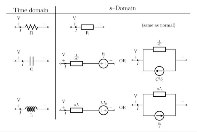
By Laplace Transform
Vc(s)= +
+
Vc(s)= +
+
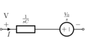
Fig 1 Laplace transformed circuit for C
Now by source conversion
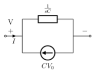
Fig 2 Source transformed circuit for C
 =
= +
+
Now if f(t)=VL(t) [voltage across inductor]
 =
= +
+
 =
= +
+
= -
- ]+
]+
= -0]+
-0]+
Multiplying both sides by 1/L

 =
= +
+
iL(t)=iL(0)+
By Laplace Transform
IL(s)= +
+
IL(s)= +
+
NOTE: Voltage------->Series circuit
Current------->Parallel circuit
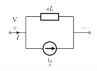
Fig 3 Laplace transformed circuit for L
By source transformation
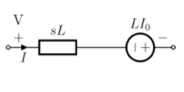
Fig 4 Source transformed circuit for L
Current through capacitor
iC(t)=
IC(s)=C[sVc(s)-Vc(0)]
Vc(s)= +
+
Voltage about inductor,
VL(t)=
VL(s)=L[sIL(s)-iL(0)]
IL(s)= +
+
Key takeaway
Vc(s)= +
+
IL(s)= +
+
Que For the given RL circuit finds the differential equation for current I.
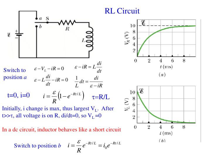
Fig5: Series RL circuit
After the switch is closed applying KVL
 =0
=0
This is a first-order homogeneous differential equation so
 dt
dt
Integrating both sides
ln i=  t+K
t+K
taking the antilog of both sides
i=k
At t=0
i(0)= =I0
=I0
 =ke0
=ke0
The particular solution is given as
i=  for t≥0
= for t<0
Ques:- Find IL(0)
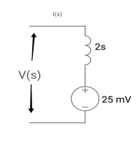
Soln: From the above circuit
L = 2H
LiL (0) = 25 mv
IL (0) = 12.5 m A
Que: Find value across the capacitor?
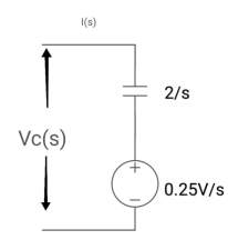
Soln:- From above circuit we can write
1/cs = 2/s
C=1/2f
Vc (0)/s = 0.25v/s
Vc(0)= .25v
Ques : Find voltage across capacitor?
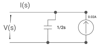
Soln:- 1/cs = 1/2S
C=2F
CVc (0) = 0.02
Vc(0)= 0.01V
Que:
switch is at before moving to position = at t= 0, at t= 0+, i1(t) is
–V/2R (b) –V/R (c) – V/4R

Sol:
I1(t) L.T I1(s)
I2(t) L.T I2(s)
then express in form
[ I1(s)/I2(s)] [::] = [:]
Drawing the ckl at t = 0-
:. The capacitor is connected for long
Vc1(0-)= V
iL(0-) =0
Vc2(0-)=0
at t= 0+

i1 (0+) = -V/2R
for t>0 the circuit is

Apply KVL
-R i1(t) -1/c  dt -L
dt -L =0
=0
Also, we can deduce i1(t)- i2 (t) = iL(t)
-Ri1(t) -1/c  - L
- L = 0
= 0
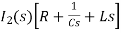
-RI1(s)-[ -
- ]-L[sI1(s)-iL(0-)]=0
- RI1(s)- -
-  -s L I2(s)=0
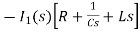 - s L I2(s)= -
  (1)
(1)
Again
-Ri2(t) ) -1/c  dt -L
dt -L =0
=0
-Ri1(t) -1/c  - L
- L = 0
= 0
Taking Laplace Transform
-RI2(s)- [ -
- ]- L[s IL(s)- iL(0-)]=0
-RI2(s)-  -
- Ls[ I1(s)- I2(s)]=0
 - s L I1(s)=0 (2)
Hence in the matrix representation
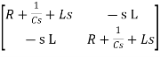
 =
= 
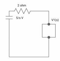
Ques: All initial conditions are zero i(t) L.T, I(s), then find I(s)?
Sol: Drawing Laplace circuit
(2+S) 11 2/S
Zeq = [(2+S)2/S]/[2+S+2/S]=[2(S+2)]/[S2+2s+2]

V1(s) = [5/S{2(S+2)/S2+2S+2}]/[2+{2(S+2)/ S2+2S+2}]
V1(s) = [5(S+2)/S]/[S2+ 3S +4]
I(s) = V1(s)/(S+2) = (5/S)/(S2+35+4)
The Laplace inverse of any function H(s) is given by
L-1 H(s) = h(t)
Properties of Inverse Laplace transform are
Linearity property
L-1 {aH1(s)+b H2(s)} = ah1(t)+bh2(t)
Shifting property
L-1 H(s) = h(t)
L-1 H(s-a) = eat h(t)
If L-1 H(s) = h(t)
Then, L-1 [H(s)/s] = 
If L-1 H(s) = h(t)
L-1 e-at H(s) = u(t-a). h(t-a)
Key takeaway

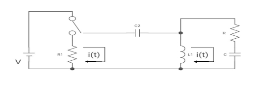
Que: The switch is at before moving to position = at t= 0, at t= 0+, i1(t) is
(a) –V/2R (b) –V/R (c) – V/4R (d) 0
Soln:-
I1(t) L.T I1(s)
I2(t) L.T I2(s)
then express in form
[ I1(s)/I2(s)] [::] .[:]
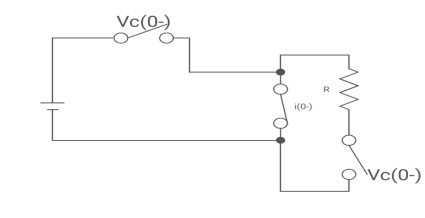
Drawing the ckl at t = 0-

Fig 6 circuit at t=0-
:. The capacitor is connected for long
Vc1(0-)= V
iL(0-) =0
Vc2(0-)=0
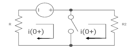
at t= 0+

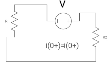
Fig 7 Circuit at t=0+
i1 (0+) = -V/2R
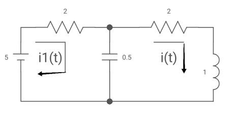
for t>0 the circuit is
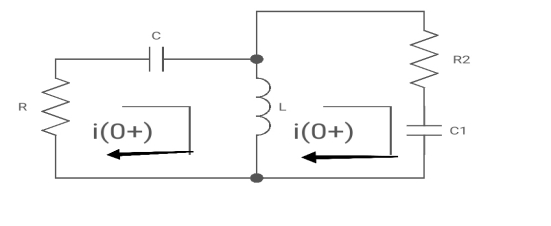
Fig 8 KVL in Circuit
Apply KVL
-R i1(t) -1/c  dt -L
dt -L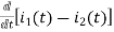 =0
=0
Also, we can deduce i1(t)- i2 (t) = iL(t)
-Ri1(t) -1/c  - L
- L = 0
= 0
-RI1(s)-[ -
- ]-L[sI1(s)-iL(0-)]=0
- RI1(s)- -
-  -s L I2(s)=0
 - s L I2(s)= -
  (1)
(1)
Again
-Ri2(t) ) -1/c  dt -L
dt -L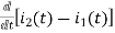 =0
=0
-Ri1(t) -1/c  - L
- L = 0
= 0
Taking Laplace Transform
-RI2(s)- [ -
- ]- L[s IL(s)- iL(0-)]=0
-RI2(s)-  -
- Ls[ I1(s)- I2(s)]=0
 - s L I1(s)=0 (2)
Hence in the matrix representation

 =
= 
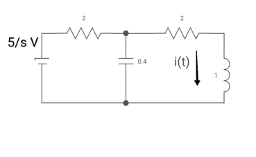
Ques: All initial conditions are zero i(t) I(s), then find I(s)?

Sol: Drawing Laplace circuit

(2+S) 11 2/S
Zeq = [(2+S)2/S]/[2+S+2/S]=[2(S+2)]/[S2+2s+2]
V1(s) = [5/S{2(S+2)/S2+2S+2}]/[2+{2(S+2)/ S2+2S+2}]
V1(s) = [5(S+2)/S]/[S2+ 3S +4]
I(s) = V1(s)/(S+2) = (5/S)/(S2+35+4)
Singularity functions are discontinuous functions or their derivatives are discontinuous. A singularity is a point at which a function does not possess a derivative. In other words, a singularity function is discontinuous at its singular points. Hence a function that is described by a polynomial in t is thus a singularity function. The commonly used singularity functions are
The convolution theorem states that f1(t) and f2(t) are two-time functions which are zero for t<0 and if Laplace transform are F1(s) and F2(s)then the transform of convolution of f1(t) and f2(t) is the product of individual transforms F1(s) and F2(s).
f(t) = f1(t)*f2(t) = 
= f2(t)*f1(t) = 
He convolution theorem of
Laplace transform is
L[f1(t)*f2(t)] = L[f2(t)*f1(t)] = F1(s)F2(s)
The Laplace Transformation transforms convolution into multiplication.
The graphical presentation of the convolution integral helps in the understanding of every step in the convolution procedure. According to the definition integral, the convolution procedure involves the following steps:
1) Apply the convolution duration property to identify intervals in which the convolution is equal to zero.
2) Flip about the vertical axis one of the signals (the one that has a simpler form (shape) since the commutativity holds), that is, represents one of the signals in the time scale.
3) Vary the parameter from - to +
to + , that is, slide the flipped signal from the left to the right, look for the intervals where it overlaps with the other signal, and evaluate the integral of the product of two signals in the corresponding intervals.
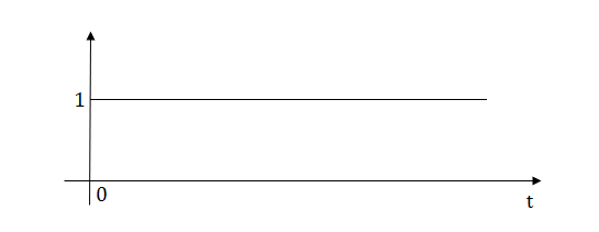
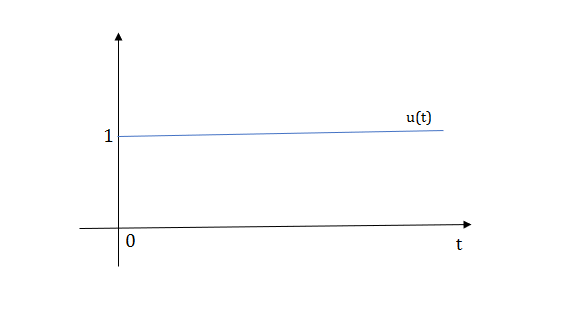
1) Step Function:
U(t)=1 t≥0
=0 t<0
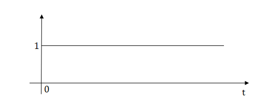
Fig 9 Step Signal

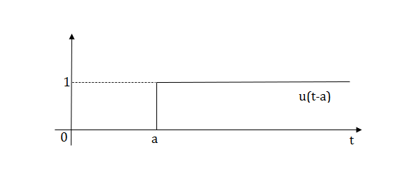
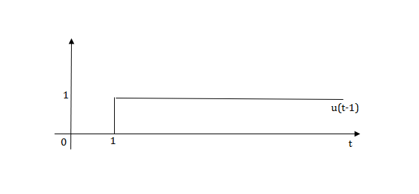
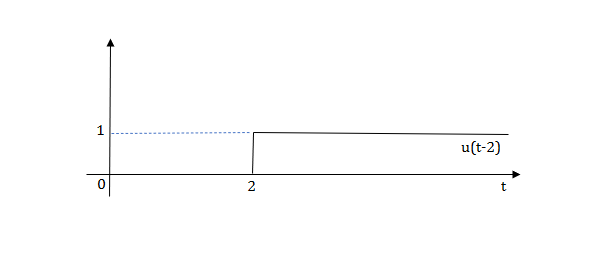
Fig 10 Shifted unit step signal
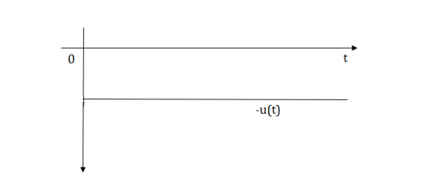
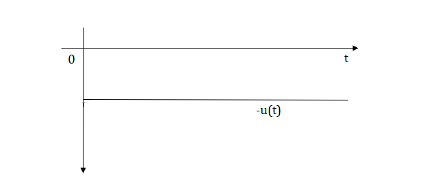
Fig 11 unit step signal -u(t)
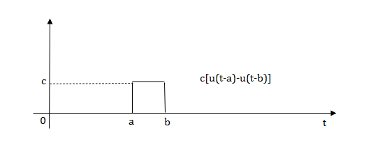
2) Pulse Function:
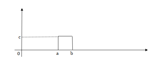
Fig 12 Pulse signal
L[u(t)]=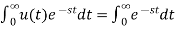 =
=
f(t)<—>F(s)
f(t-a)= F(s)
F(s)
L[u(t-a)]=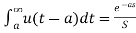
Laplace transforms of pulse
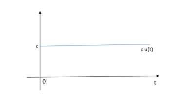
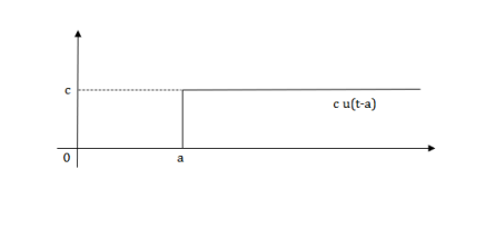
Fig 13 Shifted Pulse signal
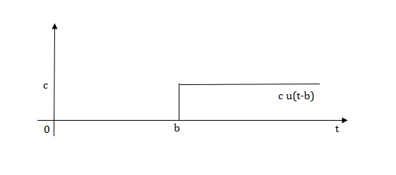
Fig 14 Shifted Pulse signal

Fig 15 Final required Pulse signal
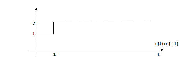
Q.1) Write an equation for a given waveform

Sol: 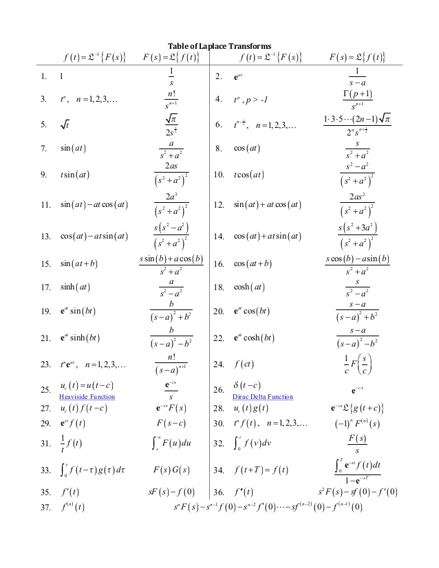

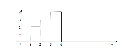
The final equation is=u(t)+u(t-1)+u(t-2)+u(t-3)-4u(t-4)
As the waveform is stopped at t=4 with amplitude 4, so we have to balance that using -4u(t-4).
Ramp function:

Fig 16 Ramp Function
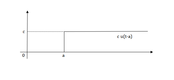
Fig 16 Shifted Ramp Function

Fig 17 Shifted Ramp Function
L[r(t)] =
R(t)=tu(t)
R(t)=∫u(t)
Impulse Signal:
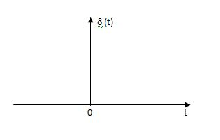 This signal has zero amplitude everywhere except at the origin. fig below showing the representation of the Impulse signal.
Fig 18 Impulse Function
The mathematical representations
A (t) = 0 for t ≠0
 dt = A e
Where A represents the energy or area of the Laplace Transform of the Impulse signal is
L [A (t) ]= A
The transfer function of a linear time-invariant system is the Laplace transform of the impulse response of the system
Q.3)Write the equation for the given waveform?
Sol: Calculating the slope of the above waveform
Slope for (0,0) and (1,2)
a1 slope= =2
=2
a2 slope= =-4
=-4

a3 slope =4 and a4= -2
At t=1 slope changes from 2 to -4 so we need to add -6r(t-1) to 2r(t) to get the slope of -4.
At t=1.5 slope changes from -4 to 4 so adding 8r(t-1.5) to get slope of 4
At t=2 slope changes from +4 to -2 so we add -6r(t-2). But we need to stop the waveform at t=3. Hence we have to make slope 0. Which can be done by adding +2r(t-3). Final equation is given as
2r(t)-6r(t-1.5)+8r(t-1.5)-6r(t-2)+2r(t-3)
Q1) Find the initial value for the function f(t) = 2u(t)+3cost u(t)?
Sol:
f(t) = 2u(t)+3cost u(t)
F(s) = 
sF(s) = 2+ 
By initial value theorem
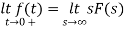 = f(0+)
 =
=  2+
2+  = 5 = f(0+)
Hence, the initial value of the function is 5
Q2) Find the final value of the function F(s) = 
Sol:
F(s) = 
sF(s) = 
By final value theorem
 =
= 
 =
=  = 0.1
= 0.1
So, the final value of the function is 0.1
Key takeaway
By initial value theorem
 = f(0+)
By final value theorem
 =
= 
Reference
[1] Network Analysis Third Edition by M. E. Van Valkenburg, Prentice Hall of India Private Limited.
[2] Network Analysis & Synthesis by G. K. Mittal, Khanna Publication.
[3] Network Analysis and Synthesis by Ravish R Singh, McGraw Hill.
[4] Introduction to Electric Circuits by Alexander & Sadiku, McGraw Hill.
[5] Introduction to Electric Circuits by S. Charkarboorty, Dhanpat Rai & Co.
[6] Fundamentals of Electrical Networks by B.R.Gupta & Vandana Singhal- S.Chand Publications
[7] Electrical Circuit Analysis 2nd Edition by P. Ramesh babu, Scitech Publication
India Pvt Ltd.


