Unit II
Searching and Sorting Algorithms
Analysis of Iterative Algorithms
Frequency count analysis for this code is as follows
Sr. No. | Instructions | Frequency count |
#include<stdio.h> |
| |
2. | #include<conio.h> |
|
3. | void main() { |
|
4. | int marks; |
|
5. | printf(“enter a marks”); | add 1 to the time count |
6. | scanf(“%d”,&marks); | add 1 to the space count |
7. | printf(“your marks is %d”,marks); | add 1 to the time count |
8. | getch(); } |
|
In the above example, for the first four instructions there is no frequency count. For data declaration and the inclusion of header file there is no frequency count. So, for this example has a frequency count for time is 2 and a frequency count for space is 1. So, total frequency count is 3.
Consider the following example
Sr. No. | Instructions | Frequency count |
#include<stdio.h> |
| |
2. | #include<conio.h> |
|
3. | void main() { |
|
4. | int sum=0; | 1 |
5. | for(i=0;i<5;i++) | 6 |
6. | sum=sum+i; | 5 |
7. | printf(“Addition is %d”,sum); | 1 |
8. | getch(); } |
|
Explanation : In the above example, one is add to frequency count for instruction four and seven after that in fifth instruction is check from zero to five so it will add value six to frequency count. ‘For’ loop executed for five times so for sixth instruction frequency count is five. Total frequency count for above program is 1+6+5+1 =13.
Consider the following example
Sr. No. | Instructions | Frequency count |
1. | #include<stdio.h> |
|
2. | #include<conio.h> |
|
3. | void main() { |
|
4. | int a[2][3],b[2][3],c[2][3]] |
|
5. | for(i=0;i<m;i++) | m+1 |
6. | { |
|
7. | for(j=0;j<n;j++) | m(n+1) |
8. | { |
|
9. | c[i][j]=a[i][j]*b[i][j]; | m.n |
10. | }} |
|
11. | getch(); } |
|
Consider the following example
Sr. No. | Instructions | Frequency count |
1. | #include<stdio.h> |
|
2. | #include<conio.h> |
|
3. | void main() { |
|
4. | int a[2][3],b[2][3],c[2][3]] |
|
5. | for(i=0;i<m;i++) | m+1 |
6. | { |
|
7. | for(j=0;j<n;j++) | m(n+1) |
8. | { |
|
9. | a[i][j]=n; | m.n |
10. | for(k=0;k<n;k++) | mn(n+1) |
11. | c[i][j]=a[i][j]*b[i][j]; | m.n.n |
12. | }} |
|
13. | getch(); } |
|
Explanation : For above program total frequency count
= (m+1)+m(n+1)+mn+mn(n+1)+mn
= m+1+mn+m+mn+mn2 +mn+mn2
= 2 mn2+3mn+2m+1
= mn(2n+3)+2m+1
Consider the following example
Sr. No. | Instructions | Frequency count |
1. | #include<stdio.h> |
|
2. | #include<conio.h> |
|
3. | void main() { |
|
4. | int n=1,m; | 1 |
5. | Do |
|
6. | { |
|
7. | printf(“hi”); | 10 |
8. | if(n==10) | 10 |
9. | break; | 1 |
10. | n++; | 9 |
11. | } |
|
12. | while(n<15); | 10 |
13. | getch(); } |
|
Explanation : the above example, one is add to frequency count for instruction four. The loop will execute till value of n is incremented to 10 from 1, so for loop statements ie instructions seven and eight is execute for tem times. when the value of ‘n’ is ten then ‘break’ statement will execute for one time and it will skip the tenth execution of tenth instruction. Tenth instruction will add value nine to frequency count. Total frequency count for above program is 10+10+1+9+10 = 40.
To express the running time complexity of algorithm three asymptotic notations are available. Asymptotic notations are also called as asymptotic bounds. Notations are used to relate the growth of complex function with the simple function. Asymptotic notations have domain of natural numbers. These notations are as follows

Fig. 3.7
In the above diagram out of two function f(n) and g(n), more complex function is f(n), so need to relate its growth as compare to simple function g(n). More specifically we need one constant function c(n) which bound function f(n) at some point n0. Beyond the point ‘n0’ function c*g(n) is always greater than f(n).
Now f(n)=Og(n)if there is some constant ‘c’ and some initial value ‘n0’. such that f(n)<=c*g(n) for all n>n0
In the above expression ‘n’ represents the input size
f(n) represents the time that algorithm will take
f(n) and g(n) are non-negative functions.
Consider the following example

Fig. 3.8
In the above example g(n) is ‘’n’ and f(n) is ‘2n+1’ and value of constant is 3. The point where c*g(n) and f(n) intersect is ‘’n0’. Beyond ‘n0’ c*g(n) is always greater than f(n) for constant ‘3’. We can write the conclusion as follows
f(n)=O g(n) for constant ‘c’ =3 and ‘n0’=1
such that f(n)<=c*g(n) for all n>n0

Fig. 3.9
In the above diagram out of two function f(n) and g(n), more complex function is f(n), so need to relate its growth as compare to simple function g(n). More specifically we need one constant function c(n) which bound function f(n) at some point n0. Beyond the point ‘n0’ function c*g(n) is always smaller than f(n).
Now f(n)=Ωg(n)if there is some constant ‘c’ and some initial value ‘n0’. such that c*g(n) <= f(n)for all n>n0
In the above expression ‘n’ represents the input size
f(n) represents the time that algorithm will take
f(n) and g(n) are non-negative functions.
Consider the following example
In the above example g(n) is ‘2n’ and f(n) is ‘2n-2’ and value of constant is 0.5. The point where c*g(n) and f(n) intersect is ‘’n0’. Beyond ‘n0’ c*g(n) is always smaller than f(n) for constant ‘0.5’. We can write the conclusion as follows
f(n) = Ω g(n) for constant ‘c’ =0.5 and ‘n0’=2
such that c*g(n)<= f(n) for all n>n0

Fig. 3.10

Fig. 3.11
In the above diagram out of two function f(n) and g(n), more complex function is f(n), so need to relate its growth as compare to simple function g(n). More specifically we need one constant function c1 and c2 which bound function f(n) at some point n0. Beyond the point ‘n0’ function c1*g(n) is always smaller than f(n) and c2*g(n) is always greater than f(n).
Now f(n) = g(n) if there is some constant ‘c1 and c2’ and some initial value ‘n0’. such that c1*g(n) <= f(n)<=c2*g(n)for all n>n0
In the above expression ‘n’ represents the input size
f(n) represents the time that algorithm will take
f(n) and g(n) are non-negative functions.
f(n) = g(n) if and only if f(n)=O g(n) and f(n)=Ω g(n)
Consider the following example

Fig. 3.12
In the above example g(n) is ‘2n’ and f(n) is ‘3n-2’ and value of constant c1 is 0.5 and c2 is 2. The point where c*g(n) and f(n) intersect is ‘’n0’. Beyond ‘n0’ c1*g(n) is always smaller than f(n) for constant ‘0.5’ and c2*g(n) is always greater than f(n) for constant ‘2’. We can write the conclusion as follows
f(n)=Ω g(n) for constant ‘c1’ =0.5 , ‘c2’ = 2 and ‘n0’=2
such that c1*g(n)<= f(n)<=c2*g(n) for all n>n0
Given a collection of objects, the goal of search is to find a particular object in this collection. The objects have key values on which search is performed and data values which correspond to the information one wishes to retrieve once an object is found. For example, a telephone book is a collection of names on which one searches and telephone numbers which correspond to the data being sought. The collection of objects is often stored in a list or an array. Given a collection of objects in an array A[1.. n], the ith element A[i] corresponds to the key value of the ith object in the collection. The input to a search algorithm is an array of objects A, the number of objects n, and the key value being sought x.
Thus Algorithm for Linear Search is
1. start at one end of the list
2. if the current element is not equal to the search target, move to the next element,
3. stop when a match is found or the opposite end of the list is reached.
Function for Linear search is
find(values, target)
{
for( i = 0; i < values.length; i++)
{
if (values[i] == target)
{ return i; }
}
return –1;
}
If element is found this function returns index of that element otherwise it returns –1.
Example : we have an array of integers, like the following:
Elements | 9 | 6 | 7 | 12 | 1 | 5 |
Index | 0 | 1 | 2 | 3 | 4 | 5 |
Let’s search for the number 7. According to function for linear search index for element 7 should be returned. We start at the beginning and check the first element in the array.
9 | 6 | 7 | 12 | 1 | 5 |
First element is 9.Match is not found and hence we move to next element i.e 6.
9 | 6 | 7 | 12 | 1 | 5 |
Again match is not found so move to next element i.e.7.
9 | 6 | 7 | 12 | 1 | 5 |
0 | 1 | 2 | 3 | 4 | 5 |
We found the match at the index position 2. Hence output is 2.
If we try to find element 10 in above array, it will return –1,as 10 is not present in the array.
Complexity Analysis of Linear Search:
Let us assume element x is to be searched in array A of size n.
An algorithm can be analyzed using following three cases.
1. Worst case
2. Average case
3. Best case
1. Worst case : In Linear search worst case happens when element to be searched is not present. When x is not present, the linear search function compares it with all the elements of A one by one. The size of A is n and hence x is to be compared with all n elements. Thus, the worst case time complexity of linear search would be O(n).
2. Average case : In average case analysis, we take all possible inputs and calculate computing time for all of the inputs. Sum all the calculated values and divide the sum by total number of inputs. Following is the value of average case time complexity.
Average Case Time = (((= ((((
= O (n)
3. Best Case : In linear search , the best case occurs when x is present at the first location. So time complexity in the best case would be O(1).
P1 : Program for Linear Search
#include<stdio.h>
#include<conio.h>
int search(int [],int, int);
void main()
{
int a[20],k,i,n,m;
clrscr();
printf(“\n\n ENTER THE SIZE OF ARRAY”);
scanf(“%d”,&n);
printf(“\n\nENTER THE ARRAY ELEMENTS\n\n”);
for(i=0;i<n;i++)
{
scanf(“%d”,&a[i]);
}
printf(“\n\nENTER THE ELEMENT FOR SEARCH\n”);
scanf(“%d”,&k);
m=search(a,n,k);
if(m==–1)
{
printf(“\n\nELEMENT IS NOT FOUND IN LIST”);
}
else
{
printf(“\n\nELEMENT IS FOUND AT LOCATION %d”,m);
}
}
getch();
}
int search(int a[],int n,int k)
{
int i;
for(i=0;i<n;i++)
{
if(a[i]==k)
{
return i;
}
}
if(i==n)
{
return –1;
}
}
Merits :
1. Simple and easy to implement
2. It works well even on unsorted arrays.
3. It is memory efficient as it does not require copying and partitioning of the array being searched.
Demerits :
Suitable only for small number of values.
It is slow as compared to binary search.
Binary Search requires sorted array.
Steps to perform binary search on sorted array A of size n are as follows.
1. Initialize lower and upper limit of array to be searched Low=0,High= n–1.
2. Find the middle position
Mid=(Low + High)/2
3. Compare the input key value with the key value of the middle element of the array. It has 3 possibilities.
Case 1 : If keys match then return mid and print element found.
if(key==A[mid])
return mid
Case 2 : If key is less than middle element then element is present in left half of array. Update High and goto step 2.
if(key<A[mid])
High= Mid–1
goto step 2
Case 3 : If key is greater than middle element then element is present in right half of array. Update Low and goto step 2.
if(key>A[mid])
Low= Mid+1
goto step 2
Case 4: if(Low>High)
Print element not found.
Iterative algorithm for Binary Search
int BinarySearch( int A[],int x)
{
int mid,n;
int Low = 0;
int High = n–1;
while ( Low <= High )
{
mid = (Low + High) / 2;
if ( A[mid] == x )
return mid;
if ( A[mid] > x )
High = mid – 1;
else Low = mid + 1;
}
return –1;
}
Example 1 : Let array A= {–1, 5, 6, 18, 19, 25, 46, 78, 102, 114}. We want to find element ‘6’ using binary search.
–1 | 5 | 6 | 18 | 19 | 25 | 46 | 78 | 102 | 114 |
0 | 1 | 2 | 3 | 4 | 5 | 6 | 7 | 8 | 9 |
Solution:
Step 1 : Low=0, High= 9
Step 2 : Mid=(Low + High)/2
Mid = (0+9)/2 =4.5 i.e 4. It means middle element is located at position 4. So A[Mid] is 19.Thus
Low=0
Mid=4
High=9
Low |
|
|
| Mid |
|
|
|
| High |
–1 | 5 | 6 | 18 | 19 | 25 | 46 | 78 | 102 | 114 |
0 | 1 | 2 | 3 | 4 | 5 | 6 | 7 | 8 | 9 |
Step 3 : Compare 6 with 19. It satisfies case 2 of step 3. so High= 4–1=3 and element is present in left half of array. We can ignore right half of array.
Repeat step 2. So mid= (0+3)/2 = 1.5 i.e 1. mid is at position 1. Element 5 is present at position 1.
Low = 0
Mid = 1
High = 3
Low | Mid |
| High |
|
–1 | 5 | 6 | 18 | 19 |
0 | 1 | 2 | 3 | 4 |
Again compare 5 with 6. It satisfies case 3 of step 3. so
Low = 1+1=2.
Repeat step 2. Mid= (2+ 3)/2= 2.5 i.e 2 .Mid is at position 2. Element 6 is at position 2.
Low=2
Mid=2
High=3
|
| Low, Mid | High |
|
|
|
|
|
|
–1 | 5 | 6 | 18 | 19 |
0 | 1 | 2 | 3 | 4 |
Compare 6 with 6.
Match is found. Return the position and print element found.
Example 2 : Find 103 in {–1, 5, 6, 18, 19, 25, 46, 78, 102, 114} using Binary Search.
Low |
|
|
| Mid |
|
|
|
| High |
–1 | 5 | 6 | 18 | 19 | 25 | 46 | 78 | 102 | 114 |
0 | 1 | 2 | 3 | 4 | 5 | 6 | 7 | 8 | 9 |
Step 1 : Low=0
High=9
Step 2 : Mid=(0+9)/2=4
So middle element is 19.
Step 3 : Compare(103,19)
103>19 hence element is located at right half of array and we can ignore left half of array. Update Low and recalculate mid.
Low = 4+1=5
High = 9
Mid = (5+9)/2=7
Low |
| Mid |
| High |
25 | 46 | 78 | 102 | 114 |
5 | 6 | 7 | 8 | 9 |
Middle element is 78. Compare(103,78)
103>78. Recalculate Low and Mid
Low = 7+1=8
High = 9
Mid = (8+9)/2=8
Low, Mid | High |
102 | 114 |
8 | 9 |
Middle element is 102. Compare(103,102)
103>102. Recalculate Low and Mid.
Low = 8+1=9
High = 9
Here Low=High and match is not found hence we conclude that element is not present in array.
Example 3 : Find 44 in A={5,12,17,23,38,44,77,84,90} using binary search.
Step 1: Low=0
High=8
Mid=(0+8)/2=4
Low |
|
|
| Mid |
|
|
| High |
5 | 12 | 17 | 23 | 38 | 44 | 77 | 84 | 90 |
0 | 1 | 2 | 3 | 4 | 5 | 6 | 7 | 8 |
Middle element is 38. Compare(44,38)
44>38.Thus element is located at right half of array and we can ignore left half of array. Recalculate Low and Mid.
Low = (4+1)= 5
High = 8
Mid = (5+8)/2=6.5 i.e 6
Low | Mid |
| high |
44 | 77 | 84 | 90 |
0 | 1 | 2 | 3 |
Middle element is 77. Compare(44,77)
44<77. Recalculate High and Mid.
Low=5
High = 6–1=5
Mid = (5+5)/2=5
Low, Mid, high |
|
|
|
44 | 77 | 84 | 90 |
0 | 1 | 2 | 3 |
Middle element is 44. Compare(44,44)
Match is Found. Return index and print “Element Found.”
Algorithm for Recursive Binary Search
int BinarySearch (int A[], int x, int Low, int High)
{
if (High > Low)
return –1;
int mid = (High + Low) / 2;
if (A[mid] == x)
return mid;
if (A[mid] < x)
return BinarySearch(A, x, mid+1, High);
return BinarySearch(A, x, Low, mid–1);
}
P2 : Program for Binary Search
#include<stdio.h>
#include<conio.h>
void main()
{
int n,i,search,f=0,low,high,mid,a[20];
clrscr();
printf("Enter the number of elements:");
scanf("%d",&n);
for(i=1;i<=n;i++)
{
printf("Enter the number in ascending order a[%d]=",i);
scanf("%d",&a[i]);
}
printf("Enter the element to be searched:");
scanf("%d",&search);
low=0;
high=n–1;
while(low<=high)
{
mid=(low+high)/2;
if(search<a[mid])
{
high=mid–1;
}
else if(search>a[mid])
{
low=mid+1;
}
else
{
f=1;
printf("Element is found at the position %d:",mid);
exit();
}
}
if(f==0)
{
printf("Element not found");
}
getch();
}
Complexity Analysis of Binary Search :
Assume our array size is 16.
When n= 16 BinarySearch is called to reduce size to n=8.
When n= 8 BinarySearch is called to reduce size to n=4.
When n= 4 BinarySearch is called to reduce size to n=2.
When n= 2 BinarySearch is called to reduce size to n=1 .
Thus we see that BinarySearch function is called 4 times
i.e. 4 elements of the array were examined for n =16.
Note that 16 = 24
Let us consider a more general case where
n is still a power of 2. Let us say n =2k
After k searches, the while loop is executed k times and n reduces to size 1. Let us assume that each run of the while loop involves at most 4 operations.
Thus total number of operations: 4k.
The value of k can be determined from the expression
2k = n
Taking log of both sides
k = log n
Thus total number of operations = 4 log n.
We conclude that the time complexity of the Binary search method is O(log n), which is much more efficient than the Linear Search method.
Merits :
Binary Search is fast and efficient.
Suitable for large number of values.
Demerits :
Binary search works only on sorted array or list.
Fibonacci series generates the subsequent number by adding two previous numbers. Fibonacci series starts from two numbers − F0 & F1. The initial values of F0 & F1 can be taken 0, 1 or 1, 1 respectively.
Fibonacci series satisfies the following conditions −
Fn = Fn-1 + Fn-2
Hence, a Fibonacci series can look like this −
F8 = 0 1 1 2 3 5 8 13
or, this −
F8 = 1 1 2 3 5 8 13 21
Fibonacci Iterative Algorithm
First we try to draft the iterative algorithm for Fibonacci series.
Procedure Fibonacci(n)
declare f0, f1, fib, loop
set f0 to 0
set f1 to 1
display f0, f1
for loop ← 1 to n
fib ← f0 + f1
f0 ← f1
f1 ← fib
display fib
end for
end procedure
Fibonacci Recursive Algorithm
Let us learn how to create a recursive algorithm Fibonacci series. The base criteria of recursion.
START
Procedure Fibonacci(n)
declare f0, f1, fib, loop
set f0 to 0
set f1 to 1
display f0, f1
for loop ← 1 to n
fib ← f0 + f1
f0 ← f1
f1 ← fib
display fib
end for
END
Steps to perform Bubble sort are as follows.
Assume we want to sort the elements in ascending order and no two elements are equal.
1. Compare first element with second element. If first element is greater than next element, we interchange their position accordingly. i.e first element is moved to second element’s position and second element is moved to first element’s position. If No, then we don’t interchange any elements.
2. The element in second position is compared with element in third position and the process of interchanging elements is performed if second is greater than third element. The whole process of comparing and interchanging is repeated till last element. When the process gets completed, the largest element in array will get placed in the last position of the array.
Let us consider array A of size n. Then Algorithm for Bubble sort is
1. Set i to 0.
2. Set j to 0.
3. if(A[j]>A[j+1])
swap A[j],A[j+1]
4. Increment j
5. if j<(n–1–i) goto step 3
6. Increment i
7. if(i<n–1) goto step 2.
Example 1 : Suppose the following numbers are stored in an array A:
32 | 51 | 27 | 85 | 66 | 23 | 13 | 57 |
j = 0 | 1 | 2 | 3 | 4 | 5 | 6 | 7 |
We apply bubble sort to array A. We discuss each pass separately.
Pass 1
1. Compare j[0] and j[1]. Since 32 < 51, the list is not altered.
2. Compare j[1] and j[2] Since 51 > 27, interchange 51 and 27 as follows:
32 | 51 | 27 | 85 | 66 | 23 | 13 | 57 |
j = 0 |
| 2 | 3 | 4 | 5 | 6 | 7 |
Array A becomes
32 | 27 | 51 | 85 | 66 | 23 | 13 | 57 |
j = 0 | 1 | 2 | 3 | 4 | 5 | 6 | 7 |
3. Compare j[2] and j[3]. Since 51 < 85, array is not altered.
4. Compare j[3] and j[4]. Since 85 > 66, interchange 85 and 66 as follows:
32 | 27 | 51 | 85 | 66 | 23 | 13 | 57 |
j = 0 | 1 | 2 | 3 | 4 | 5 | 6 | 7 |

Array A becomes
32 | 27 | 51 | 66 | 85 | 23 | 13 | 57 |
j = 0 | 1 | 2 | 3 | 4 | 5 | 6 | 7 |
5. Compare j[4] and j[5]. Since 85 > 23, interchange 85 and 23 as follows:
32 | 27 | 51 | 66 | 85 | 23 | 13 | 57 |
j = 0 | 1 | 2 | 3 | 4 | 5 | 6 | 7 |

Array A becomes
32 | 27 | 51 | 66 | 23 | 85 | 13 | 57 |
j = 0 | 1 | 2 | 3 | 4 | 5 | 6 | 7 |
6. Compare j[5] and j[6]. Since 85 > 13, interchange 85 and 13 as follows:
32 | 27 | 51 | 66 | 23 | 85 | 13 | 57 |
j = 0 | 1 | 2 | 3 | 4 | 5 | 6 | 7 |

32 | 27 | 51 | 66 | 23 | 13 | 85 | 57 |
j = 0 | 1 | 2 | 3 | 4 | 5 | 6 | 7 |
7. Compare j[6] and j[7]. Since 85 > 57, interchange 85 and 57 as follows:
32 | 27 | 51 | 66 | 23 | 13 | 85 | 57 |
j = 0 | 1 | 2 | 3 | 4 | 5 | 6 | 7 |

Array A becomes
32 | 27 | 51 | 66 | 23 | 13 | 57 | 85 |
j = 0 | 1 | 2 | 3 | 4 | 5 | 6 | 7 |
At the end of this first pass, the largest number, 85, has moved to the last position. However, the rest of the numbers are not sorted, even though some of them have changed their positions.
Pass 2 will move second last number at second last position, Pass 3 will move third last number at third last position and so on. Here we show array after every pass.
Pass 2 :
27 | 33 | 51 | 23 | 13 | 57 | 66 | 85 |
j = 0 | 1 | 2 | 3 | 4 | 5 | 6 | 7 |
Pass 3 :
27 | 33 | 23 | 13 | 51 | 57 | 66 | 85 |
j = 0 | 1 | 2 | 3 | 4 | 5 | 6 | 7 |
Pass 4:
27 | 23 | 13 | 33 | 51 | 57 | 66 | 85 |
j = 0 | 1 | 2 | 3 | 4 | 5 | 6 | 7 |
Pass 5 :
23 | 13 | 27 | 33 | 51 | 57 | 66 | 85 |
j = 0 | 1 | 2 | 3 | 4 | 5 | 6 | 7 |
Pass 6 :
13 | 23 | 27 | 33 | 51 | 57 | 66 | 85 |
j = 0 | 1 | 2 | 3 | 4 | 5 | 6 | 7 |
Hence the array is sorted in 6 passes.
We will see one more example
Example 2 : Apply Bubble Sort on array A= {5,3,1,9,8,2,4,7}.
j =0 | 5 | 3 | 1 | 9 | 8 | 2 | 4 | 7 |
j =1 | 3 | 5 | 1 | 9 | 8 | 2 | 4 | 7 |
j =2 | 3 | 1 | 5 | 9 | 8 | 2 | 4 | 7 |
j =3 | 3 | 1 | 5 | 9 | 8 | 2 | 4 | 7 |
j =4 | 3 | 1 | 5 | 8 | 9 | 2 | 4 | 7 |
j =5 | 3 | 1 | 5 | 8 | 2 | 9 | 4 | 7 |
j =6 | 3 | 1 | 5 | 8 | 2 | 4 | 9 | 7 |
j =7 | 3 | 1 | 5 | 8 | 2 | 4 | 7 | 9 |
Pass 2 : i=2
3 | 1 | 5 | 8 | 2 | 4 | 7 | 9 |
1 | 3 | 5 | 8 | 2 | 4 | 7 | 9 |
1 | 3 | 5 | 8 | 2 | 4 | 7 | 9 |
1 | 3 | 5 | 8 | 2 | 4 | 7 | 9 |
1 | 3 | 5 | 2 | 8 | 4 | 7 | 9 |
1 | 3 | 5 | 2 | 4 | 8 | 7 | 9 |
1 | 3 | 5 | 2 | 4 | 7 | 8 | 9 |
Pass 3 :
1 | 3 | 5 | 2 | 4 | 7 | 8 | 9 |
1 | 3 | 5 | 2 | 4 | 7 | 8 | 9 |
1 | 3 | 5 | 2 | 4 | 7 | 8 | 9 |
1 | 3 | 2 | 5 | 4 | 7 | 8 | 9 |
1 | 3 | 2 | 4 | 5 | 7 | 8 | 9 |
Pass 4 :
1 | 3 | 2 | 4 | 5 | 7 | 8 | 9 |
1 | 3 | 2 | 4 | 5 | 7 | 8 | 9 |
1 | 2 | 3 | 4 | 5 | 7 | 8 | 9 |
This array gets sorted in 4 passes only.
Example : Apply Bubble Sort on array A= {23,78,45,8,32,56}
Pass 1 :
23 | 78 | 45 | 8 | 32 | 56 |
23 | 78 | 45 | 8 | 32 | 56 |
23 | 45 | 78 | 8 | 32 | 56 |
23 | 45 | 8 | 78 | 32 | 56 |
23 | 45 | 8 | 32 | 78 | 56 |
23 | 45 | 8 | 32 | 56 | 78 |
Pass 2 :
23 | 45 | 8 | 32 | 56 | 78 |
23 | 45 | 8 | 32 | 56 | 78 |
23 | 8 | 45 | 32 | 56 | 78 |
23 | 8 | 32 | 45 | 56 | 78 |
Pass 3 :
23 | 8 | 32 | 45 | 56 | 78 |
8 | 23 | 32 | 45 | 56 | 78 |
This array is sorted in 3 passes.
P3: Write a Program for Bubble sort in C
#include <stdio.h>
#include<conio.h>
void bubble_sort(int A[], int n);
int main()
{
int A[100], n, i, j, swap;
printf("Enter number of elements\n");
scanf("%d", &n);
printf("Enter the elements\n", );
for (i = 0; i < n; i++)
scanf("%d", &A[i]);
bubble_sort(A, n);
printf("Sorted list in ascending order:\n");
for ( i = 0 ; i < n ; i++ )
printf("%ld\n", A[i]);
return 0;
}
void bubble_sort(int A[], int n)
{
int i, j, t;
for (i = 0 ; i < ( n – 1 ); i++)
{
for (j = 0 ; j < (n – i – 1); j++)
{
if (A[j] > list[j+1])
{
/* Swapping */
t = A[j];
A[j] = A[j+1];
A[j+1] = t;
}
}
}
}
Complexity Bubble sort:
Suppose we have a list with n elements, and each element perform n – 1 comparisons with elements to its left, and swap, if necessary.
Best Case: If the list is already sorted, only one iteration is performed and complexity is O(1).
Average and Worst case: For n elements at most n – 1 swap operations is performed in each pass. The worst and average case complexity is O(n2).
Insertion Sort reads all elements from 1 to n and inserts each element at its proper position. This sorting method works well on small list of elements.
Procedure for each pass is as follows.
Pass 1 :
A[l] by itself is trivially sorted.
Pass 2 :
A[2] is inserted either before or after A[l] so that: A[l], A[2] is sorted.
Pass 3 :
A[3] is inserted into its proper place so that: A[l], A[2], A[3] is sorted.
Pass 4 :
A[4] is inserted into its proper place A[l], A[2], A[3], A[4] is sorted.
Pass N :
A[N] is inserted into its proper place in so that:
A[l], A[ 2 ] , . . . , A[ N ] is sorted
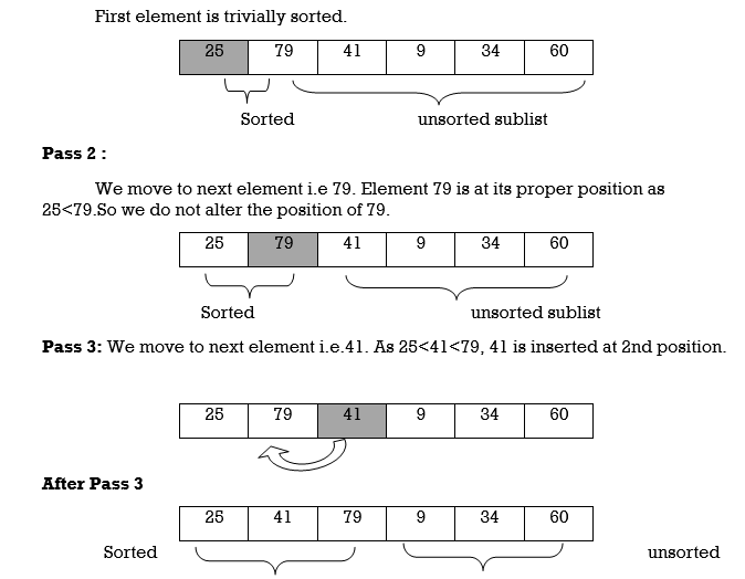
Example : We will apply insertion sort on original list of Fig.3.Assume we are arranging elements in ascending order.
25 | 79 | 41 | 9 | 34 | 60 |
Fig.: Original List
Pass 1 :
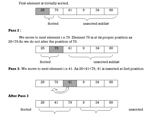
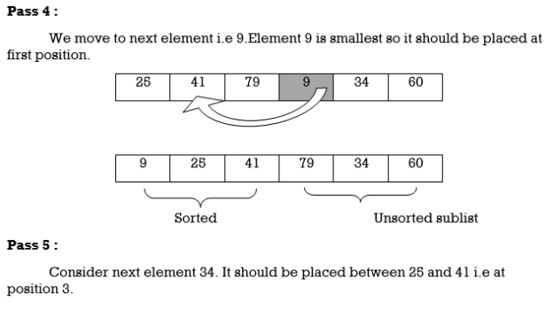
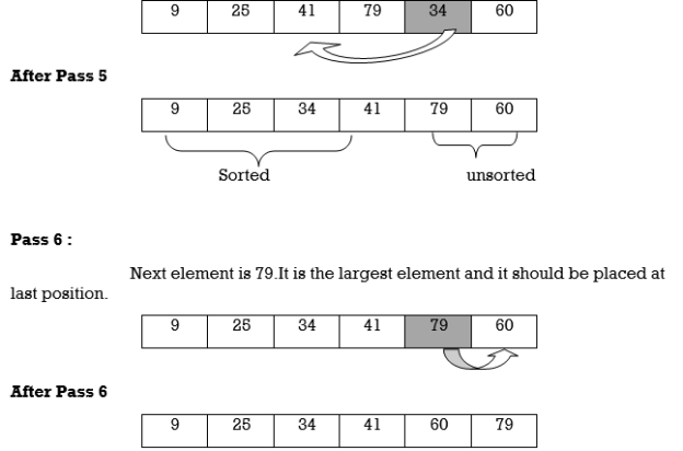 Hence the list is sorted using insertion sort.
We will see one more example.
Apply Insertion sort on array A= {77,30,40,10,88,20,65,56}
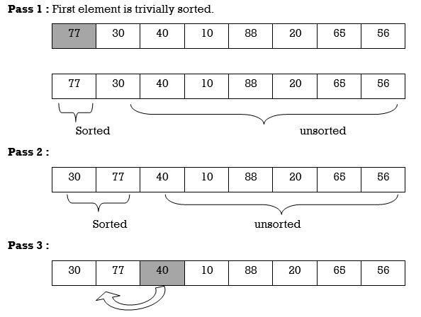
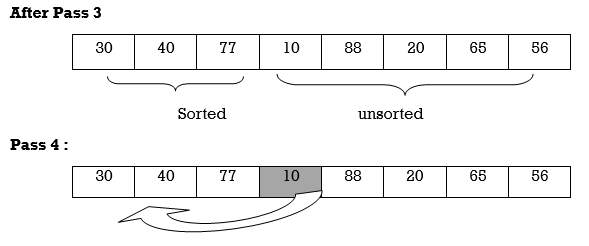
After Pass 4
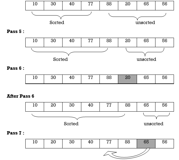
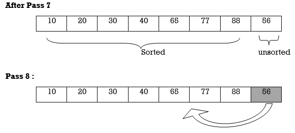
After Pass 8
10 | 20 | 30 | 40 | 56 | 65 | 77 | 88 |
Hence the list is sorted using Insertion sort.
C Function for Insertion Sort
void insertionSort(int A[], int n)
{
int i, p, temp, j;
for (i = 1; i<=n; i++)
{
p= 0;
temp = A[i];
for (j=i–1; j >= 0 && !p;)
if(temp < A[j])
{
A[j + 1]= A[j];
j––;
}
else
p = 1;
A[j + 1] = temp;
}
return;
}
P5 : Program to implement insertion sort.
#include <stdio.h>
int main()
{
int n, A[100], i, j, t;
printf("Enter number of elements\n");
scanf("%d", &n);
printf("Enter %d integers\n", n);
for (i = 0; i < n; i++) {
scanf("%d", &A[i]);
}
for (i = 1 ; i <=( n – 1); i++)
{
j = i;
while ( j > 0 && A[j] < A[j–1])
{
t = A[j];
A[j] = A[j–1];
A[j–1] = t;
j––;
}
}
printf("Sorted list in ascending order:\n");
for (i = 0; i <= n – 1; i++) {
printf("%d\n", A[i]);
}
return 0;
}
Output :
Enter number of elements
5
Enter 5 integers
9
4
2
5
3
Sorted list in ascending order
2
3
4
5
9
Complexity of Insertion Sort :
Worst Case Complexity: In the worst case, for each i we do (i – 1) swaps inside the inner for–loop–therefore, overall number of swaps (when i goes from 2 to n in the outer for loop) is
T(n) = 1 + 2 + 3 +...+(I – 1) +....+ n – 1
= n (n – 1)/2
= O(n2)
Average case Complexity is O(n2).
Best Case Complexity is O(n).
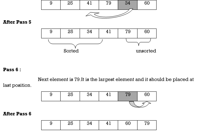
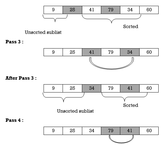
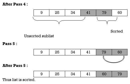
Assume we want to sort list in ascending order. Selection sort finds the smallest element from unsorted list and swap it with the element in first position. Then it finds second smallest element and swap it with element at second position. This process is repeated till entire list is sorted in ascending order. Each time we swap elements, we say that we have completed a sort pass. A list of n elements requires n–1 passes to completely rearrange the data.
Procedure for every pass is as follows.
Pass 1 : Find the position P of the smallest in the list of N elements A[l], A[2], . . . , A[N], and then interchange A[P] and A[1] . Then A[1] is sorted.
Pass 2 : Find the position P of the smallest in the sublist of N –1 elements A[2], A[3],. . . , A[N], and then interchange A[P]and A[2]. Then A[l], A[2] is sorted.
Pass 3 : Find the position P of the smallest in the sublist of N–2 elements A[3], A[4], . . . , A[N], and then interchange A[P] and A[3]. Then: A[l], A[2] , A[3] is sorted.
Pass N –1 : Find the position P of the smaller of the elements A[N –1), A[N], and then interchange A[P] and A[N–1]. Then: A[l], A[2], . . . , A[N] is sorted. Thus A is sorted after N –1 passes.
Example 1 :
25 | 79 | 41 | 9 | 34 | 60 |
Fig.: Original List
We will apply selection sort on this list.
After Pass 2 :

We will see one more example.
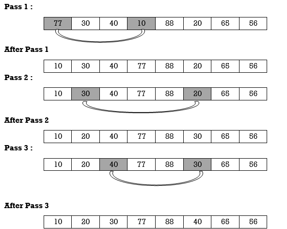
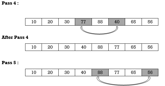
Apply selection sort on array A= {77,30,40,10,88,20,65,56}


After Pass 6
10 | 20 | 30 | 40 | 56 | 65 | 77 | 88 |
Hence the list is sorted in ascending order by applying selection sort.
Function for Selection Sort
void selectionSort(int A[], int n)
{
int i, j, s, temp;
for (i= 0; i <= n; i ++)
{
s = i;
for (j=i+1; j <= n; j++)
if(A[j] < A[s])
s= j;
// Smallest selected; swap with current element
temp = A[i];
A[i] = A[s];
A[s] = temp;
}
P4 : Program to perform Selection Sort.
#include <stdio.h>
int main()
{
int A[100], n, i, j, s, temp;
/* n=total no. of elements in array
s= smallest element in unsorted array
temp is used for swapping */
printf("Enter number of elements\n");
scanf("%d", &n);
printf("Enter %d integers\n", n);
for ( i = 0 ; i < n ; i++ )
scanf("%d", &A[i]);
for ( i = 0 ; i < ( n – 1 ) ; i++ )
{
s = i;
for ( j = i + 1 ; j < n ; j++ )
{
if ( A[s] > A[j] )
s = j;
}
if ( s != i )
{
temp = A[i];
A[i] = A[s];
A[s] = temp;
}
}
printf("Sorted list in ascending order:\n");
for ( i = 0 ; i < n ; i++ )
printf("%d\n", A[i]);
return 0;
}
Output:
Enter number of elements
5
Enter 5 integers
4
1
7
5
9
Sorted list in ascending order
1
4
5
7
9
Complexity of Selection Sort :
In selection sort outer for loop is executed n–1 time. On the kth time through the outer loop, initially the sorted list holds
k–1 elements and unsorted portion holds n–k+1 element. In inner for loop 2 elements are compared each time.
Thus, 2*(n–k) elements are examined by the inner loop during the k th pass through the outer loop. But k ranges from 1 to n–1.
Total number of elements examined is:
T(n) = 2*(n –1) + 2*(n–2) + 2*(n–3) + .. + 2*(n–(n–2))
+ 2*(n–(n–1))
= 2*((n–1) + (n–2) + (n–3) + ... + 2 + 1)
(or 2*(sum of first n–1 integers)
= 2*((n–1)*n)/2)
= n2 – n, so complexity of algorithm is O(n2).
Merge Sort is based on divide and conquer strategy. It divides the unsorted list into n sublists such that each sublist contains one element. Each sublist is then sorted and merged until there is only one sublist.
Step 1 : Divide the list into sublists such that each sublist contains only one element.
Step 2 : Sort each sublist and Merge them.
Step 3 : Repeat Step 2 till the entire list is sorted.
Example : Apply Merge Sort on array A= {85,24,63,45,17,31,96,50}
Step1 : A contains 8 elements. First we divide the list into two sublists such that each sublist contains 4 elements. Then we divide each sublist of 4 elements into sublist of two elements each. Finally every sublist contains only one element.

Fig. 4.4
Step 2 : Now we start from bottom. Compare 1st and 2nd element. Sort and merge them. Apply this for all bottom elements.
Thus we got 4 sublists as follows
24 | 85 |
| 45 | 63 |
| 17 | 31 |
| 50 | 96 |
Step 3 : Repeat this sorting and merging until entire list is sorted. Thus above four sublists are sorted and merged to form 2 sublists.
24 | 85 | 63 | 85 |
| 17 | 31 | 50 | 96 |
Finally above 2 sublists are again sorted and merged in one sublist.
17 | 24 | 31 | 45 | 50 | 63 | 85 | 96 |
We will see one more example on merge sort.
Example : Apply merge Sort on array A={10,5,7,6,1,4,8,3,2,9,12,11}
Step 1 :
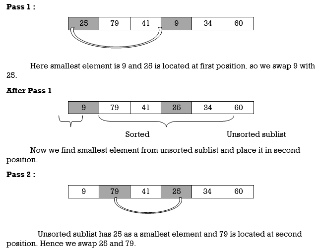
Fig. 4.5
Algorithm for Merge Sort:
Let x = no. of elements in array A
y = no. of elements in array B
C = sorted array with no. of elements n
n = x+y
Following algorithm merges a sorted x element array A and sorted y element array B into a sorted array C, with n = x + y elements. We must always keep track of the locations of the smallest element of A and the smallest element of B which have not yet been placed in C. Let LA and LB denote these locations, respectively. Also, let LC denote the location in C to be filled. Thus, initially, we set
LA : = 1,
LB : = 1 and
LC : = 1.
At each step , we compare A[LA] and B[LB] and assign the smaller element to C[LC].
Then
LC:= LC + 1,
LA: = LA + 1, if new element has come from A .
LB: = LB + 1, if new element has come from B.
Furthermore, if LA> x, then the remaining elements of B are assigned to C;
 LB >y, then the remaining elements of A are assigned to C.
Thus the algorithm becomes
MERGING ( A, x, B, y, C)
1. [Initialize ] Set LA : = 1 , LB := 1 AND LC : = 1
2. [Compare] Repeat while LA <= x and LB <= y
If A[LA] < B[LB] , then
(a) [Assign element from A to C ] set C[LC] = A[LA]
(b) [Update pointers ] Set LC := LC +1 and LA = LA+1
Else
(a) [Assign element from B to C] Set C[LC] = B[LB]
(b) [Update Pointers] Set LC := LC +1 and LB = LB +1
[End of loop]
3. [Assign remaining elements to C]
If LA > x , then
Repeat for K= 0 ,1,2,........,y–LB
Set C[LC+K] = B[LB+K]
[End of loop]
Else
Repeat for K = 0,1,2,......,x–LA
Set C[LC+K] = A[LA+K]
[End of loop]
4. Exit
Program for Merge Sort
#include<stdio.h>
#define MAX 50
void mergeSort(int A[],int first,int mid,int high);
void divide(int A[],int first,int last);
int main(){
int merge[MAX],i,n;
printf("Enter the total number of elements: ");
scanf("%d",&n);
printf("Enter the elements which to be sort: ");
for(i=0;i<n;i++){
scanf("%d",&merge[i]);
}
divide(merge,0,n–1);
printf("After merge sorting elements are: ");
for(i=0;i<n;i++){
printf("%d ",merge[i]);
}
return 0;
}
void divide(int A[],int first, int last)
{
int mid;
if(first<last){
mid=(first+last)/2;
divide(A,first,mid);
divide(A,mid+1,last);
mergeSort(A,first,mid,last);
}
}
void mergeSort(int A[],int first,int mid,int last)
{
int i,m,k,l,temp[MAX];
l=first;
i=first;
m=mid+1;
while((l<=mid)&&(m<=last)){
if(A[l]<=A[m]){
temp[i]=A[l];
l++;
}
else{
temp[i]=A[m];
m++;
}
i++;
}
if(l>mid){
for(k=m;k<=last;k++){
temp[i]=arr[k];
i++;
}
}
else{
for(k=l;k<=mid;k++){
temp[i]=arr[k];
i++;
}
}
for(k=first;k<=last;k++){
A[k]=temp[k];
}
}
Output :
Enter the total number of elements: 5
Enter the elements which to be sort: 3 1 6 4 7
After merge sorting elements are: 1 3 4 6 7
Complexity of Merge Sort :
Time to merge sort N elements = Time to merge sort N/2 elements plus time to merge two arrays each N/2 elements.
Time to merge two arrays each N/2 elements is linear, i.e. N
Thus we have:
(1) T(1) = 1
(2) T(N) = 2T(N/2) + N
Dividing (2) by N we get:
(3) T(N) / N = T(N/2) / (N/2) + 1
N is a power of two, so we can write
(4) T(N/2) / (N/2) = T(N/4) / (N/4) +1
(5) T(N/4) / (N/4) = T(N/8) / (N/8) +1
(6) T(N/8) / (N/8) = T(N/16) / (N/16) +1
(7) ……
(8) T(2) / 2 = T(1) / 1 + 1
Adding equations (3) through (8), the sum of their left–hand sides will be equal to the sum of their right–hand sides:
T(N) / N + T(N/2) / (N/2) + T(N/4) / (N/4) + … + T(2)/2
= T(N/2) / (N/2) + T(N/4) / (N/4) + ….+ T(2) / 2 + T(1) / 1 + LogN
(LogN is the sum of 1s in the right–hand sides)
After crossing the equal term, we get
(9) T(N)/N = T(1)/1 + LogN
T(1) is 1, hence we obtain
(10) T(N) = N + NlogN = O(NlogN)
Hence the complexity of the Merge Sort algorithm is O(NlogN).
Quick sort is most efficient method of sorting .It uses divide and conquer strategy to sort the elements. In quicksort, we divide the array of items to be sorted into two partitions and then call the quicksort procedure recursively to sort the two partitions. For this we choose a pivot element and arrange all elements such that all the elements in the left part are less than the pivot and all those in the right part are greater than it.
Algorithm to implement Quick Sort is as follows.
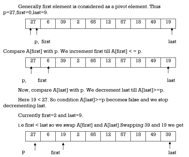
Consider array A of size n to be sorted. p is pivot element. Index positions of first and last element of array A is denoted by ‘first’ and ‘last’.
Initially first=0 and last=n–1.
Increment first till A[first]<=p
Decrement last till A[last]>=p
If first < last then swap A[first] with A[last].
If first > last then swap p with A[last] and thus position of p is found. Pivot p is placed such that all elements to its left are less than it and all elements right to it are greater than it. Let us assume that j is final position of p. Then A[0] to A[j–1] are less than p and A [j + 1] to A [n–1]are greater than p.
Now we consider left part of array A i.e A[0] to A[j–1].Repeat step 1,2,3 and 4. Apply same procedure for right part of array.
We continue with above steps till no more partitions can be made for every subarray.
C function for Quick sort
x=0,y=n–1
void Quicksort(A,x,y)
{
if(x<y)
{
first=x;
last=y;
p=A[x];
while(first<last)
{
while(A[first]<p)
first++;
while(A[last]>p)
last ––;
if(first<last)
swap(A[first],A[last])
}
swap(A[x],A[y])
Quicksort(A,x,last–1);
Quicksort(A,first+1,y);
}
We will see examples on Quick sort
Example : Apply Quicksort on array
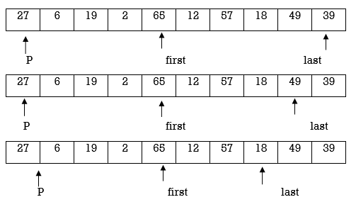
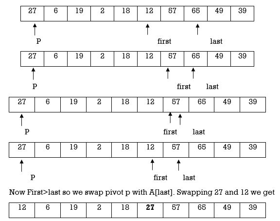
A= {27,6,39,2,65,12,57,18,49,19}
Pass 1 :
Here again first<last so we swap A[first] and A[last]. Swapping 65 and 18 we get


Here we complete Pass 1.Now pivot element is 27 and it divides array in left and right partition. We can see that elements less than pivot are in left partition and elements greater than pivot are in right partition.
Now we continue same procedure for left and right partition. Here we see results of corresponding passes.
Pass 2 :
12 | 6 | 19 | 2 | 18 | 27 | 57 | 65 | 49 | 39 |
Pass 3 :
2 | 6 | 12 | 19 | 18 | 27 | 57 | 65 | 49 | 39 |
Pass 4 :
2 | 6 | 12 | 18 | 19 | 27 | 57 | 65 | 49 | 39 |
Pass 5 :
2 | 6 | 12 | 18 | 19 | 27 | 49 | 39 | 57 | 65 |
Pass 6 :
2 | 6 | 12 | 18 | 19 | 27 | 39 | 49 | 57 | 65 |
Pass 7 :
2 | 6 | 12 | 18 | 19 | 27 | 39 | 49 | 57 | 65 |
We will see another example.
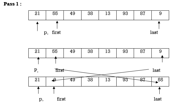
Example : Apply Quicksort on array A={21,55,49,38,13,93,87,9}

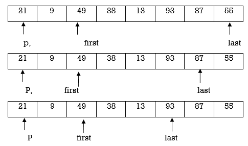
Now first>last hence swap pivot and A[last].Swapping 21 and 13 we get
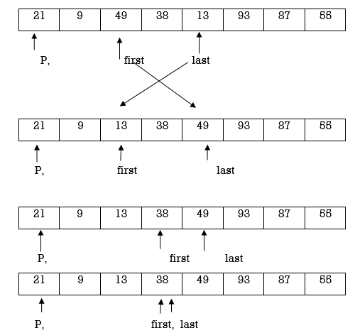
Now first > last hence swap pivot and A [last]’. Swapping 21 and 13 we get
Left Partition
13 | 9 |
P, first | last |

Hence the left partition is sorted.
Considering right partition
38 | 49 | 93 | 87 | 55 |
P, first |
|
|
| last |
38 | 49 | 93 | 87 | 55 |
P, | First |
|
| last |
38 | 49 | 93 | 87 | 55 |
Hence the right partition is sorted .
Final sorted array is
9 | 13 | 21 | 38 | 49 | 55 | 87 | 93 |
Example : Apply Quick Sort on A={42,15,9,75,18,2,55,1,64}
42 | 15 | 9 | 75 | 18 | 2 | 55 | 1 | 64 |
P, first |
|
|
|
|
|
|
| Last |
42 | 15 | 9 | 75 | 18 | 2 | 55 | 1 | 64 |
P | First |
|
|
|
|
|
| Last |
42 | 15 | 9 | 75 | 18 | 2 | 55 | 1 | 64 |
P |
| First |
|
|
|
|
| Last |
42 | 15 | 9 | 75 | 18 | 2 | 55 | 1 | 64 |
P |
|
| First |
|
|
|
| Last |

42 | 15 | 9 | 1 | 18 | 2 | 55 | 75 | 64 |
P |
|
|
| First |
|
| last |
|
42 | 15 | 9 | 1 | 18 | 2 | 55 | 75 | 64 |
P |
|
|
|
| first |
| last |
|
42 | 15 | 9 | 1 | 18 | 2 | 55 | 75 | 64 |
P |
|
|
|
|
| first | last |
|
42 | 15 | 9 | 1 | 18 | 2 | 55 | 75 | 64 |
P |
|
|
|
|
| first, last |
| |
42 | 15 | 9 | 1 | 18 | 2 | 55 | 75 | 64 |
P |
|
|
|
| Last | first |
|
|
Swap p and A[last]

Applying Quick sort on left partition
2 | 15 | 9 | 1 | 18 |
P, first |
|
|
| Last |
2 | 15 | 9 | 1 | 18 |
P | First |
| Last |
|

2 | 1 | 9 | 15 | 18 |
P |
| First | Last |
|
2 | 1 | 9 | 15 | 18 |
P |
| First, Last |
| |
2 | 1 | 9 | 15 | 18 |
P | Last | First |
|
|
As first>last swap p and A[last]
1 | 2 | 9 | 15 | 18 |
Left partition is sorted.
Apply Quicksort on right partition
55 | 75 | 64 |
P, first |
| last |
55 | 75 | 64 |
P | First | last |
55 | 75 | 64 |
P | First, last | |
55 | 75 | 64 |
P, last | First |
|
75 | 64 | |
P, First | Last | |
75 | 64 | |
P | First, last | |
75 | 64 |
P, last | First |
64 | 75 |
Hence the right partition is sorted.
Sorted array is
1 | 2 | 9 | 15 | 18 | 42 | 55 | 64 | 75 |
Program for Quick Sort:
#include<stdio.h>
void quicksort(int A[10],int,int);
int main(){
int A[20],n,i;
printf("Enter size of the array: ");
scanf("%d",&n);
printf("Enter %d elements: ",n);
for(i=0;i<n;i++)
scanf("%d",&A[i]);
quicksort(A,0,n–1);
printf("Sorted elements: ");
for(i=0;i<n;i++)
printf(" %d",A[i]);
return 0;
}
void quicksort(int A[20],int first, int last)
{
int pivot,j,temp,i;
if(first<last){
pivot=first;
i=first;
j=last;
while(i<j){
while(A[i]<=A[pivot]&&i<last)
i++;
while(A[j]>A[pivot])
j––;
if(i<j){
temp=A[i];
A[i]=A[j];
A[j]=temp;
}
}
temp=A[pivot];
A[pivot]=A[j];
A[j]=temp;
quicksort(A,first,j–1);
quicksort(A,j+1,last);
}
}
Output :
Enter size of the array: 5
Enter 5 elements: 3 8 0 1 2
Sorted elements: 0 1 2 3 8
Complexity of Quick Sort
The time to sort the file is equal to
the time to sort the left partition with i elements, plus
the time to sort the right partition with N–i–1 elements, plus
the time to build the partitions
Worst case analysis
The pivot is the smallest element
T(N) = T(N – 1) + cN, N > 1
T(N – 1) = T(N – 2) + c(N – 1)
T(N – 2) = T(N – 3) + c(N – 2)
T(N – 3) = T(N – 4) + c(N– 3)
T(2) = T(1) + c.2
Add all equations:
T(N) + T(N – 1) + T(N – 2) + … + T(2) =
= T(N – 1) + T(N – 2) + … + T(2) + T(1) + c(N) + c(N – 1) + c(N – 2) + … + c.2
T(N) = T(1) + c times (the sum of 2 thru N) = T(1) + c(N(N+1)/2 –1) = O(N2)
Best–case analysis:
The pivot is in the middle
T(N) = 2T(N/2) + cN
Divide by N:
T(N) / N = T(N/2) / (N/2) + c
T(N/2) / (N/2) = T(N/4) / (N/4) + c
T(N/4) / (N/4) = T(N/8) / (N/8) + c
…..
T(2) / 2 = T(1) / (1) + c
Add all equations:
T(N) / N + T(N/2) / (N/2) + T(N/4) / (N/4) + …. + T(2) / 2
= (N/2) / (N/2) + T(N/4) / (N/4) + … + T(1) / (1) + c.logN
After crossing the equal terms:
T(N)/N = T(1) + cLogN
T(N) = N + NcLogN = O(NlogN)
Average case analysis
Similar computations, resulting in T(N) = O(NlogN)
The average value of T(i) is 1/N times the sum of T(0) through T(N–1)
1/N S T(j), j = 0 thru N–1
T(N) = 2/N (S T(j)) + cN
Multiply by N
NT(N) = 2(S T(j)) + cN*N
To remove the summation, we rewrite the equation for N–1:
(N–1)T(N–1) = 2(S T(j)) + c(N–1)2, j = 0 thru N–2
and subtract:
NT(N) – (N–1)T(N–1) = 2T(N–1) + 2cN –c
NT(N) = (N+1)T(N–1) + 2cN
Divide by N(N+1):
T(N)/(N+1) = T(N–1)/N + 2c/(N+1)
T(N)/(N+1) = T(N–1)/N + 2c/(N+1)
T(N–1)/(N) = T(N–2)/(N–1)+ 2c/(N)
T(N–2)/(N–1) = T(N–3)/(N–2) + 2c/(N–1)
….
T(2)/3 = T(1)/2 + 2c /3
Add the equations and cross equal terms:
T(N)/(N+1) = T(1)/2 +2c S (1/j), j = 3 to N+1
The sum S (1/j), j =3 to N–1, is about LogN
Thus T(N) = O(NlogN)
Reference Books:
1. E Balgurusamy, “Programming in ANSI C”, Tata McGraw-Hill, 3rd Edition.
2. Yedidyah Langsam, Moshe J Augenstein and Aaron M Tenenbaum “Data structures using C and C++” PHI Publications, 2nd Edition.
3. Reema Thareja, “Data Structures using C”, Oxford University Press, 2
nd Edition.
