Unit V
Trees
A tree data structure can be defined recursively (locally) as a collection of nodes (starting at a root node), where each node is a data structure consisting of a value, together with a list of references to nodes (the "children"), with the constraints that no reference is duplicated, and none points to the root.
Definition of TREE:
A tree is defined as a set of one or more nodes T such that:
There is a specially designed node called root node
The remaining nodes are partitioned into N disjoint set of nodes T1, T2,…..Tn, each of which is a tree.

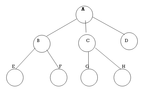
Fig. Example of tree
In above tree A is Root.
Remaining nodes are partitioned into three disjoint sets:
{B, E, F}, {C, G, H}, {D}.
All these sets satisfies the properties of tree.
Some examples of TREE and NOT TREE
Each linear list is trivially a tree

Not a tree: cycle A→A

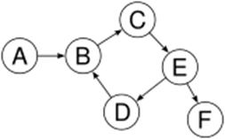
Not a tree: cycle B→C→E→D→B
Not a tree: two non-(connected parts, A→B and C→D→E
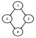
Not a tree: undirected cycle 1-2-4-3
Fig. Examples of tree and no tree
A binary tree is a special cas eof tree in which no node of a tree can have degree more than two.
Definition of Binary Tree:
A binary tree is made of nodes, where each node contains a "left" pointer, a "right" pointer, and a data element. The "root" pointer points to the topmost node in the tree. The left and right pointers recursively point to smaller "subtrees" on either side. A null pointer represents a binary tree with no elements -- the empty tree.
The formal recursive definition is A binary tree is either empty (represented by a null pointer), or is made of a single node, where the left and right pointers (recursive definition ahead) each point to a binary tree.
Example of Binary Tree:

Fig. Example of Binary Tree
Tree Terminologies
Representation
There are many different ways to represent trees; common representations represent the nodes as dynamically allocated records with pointers to their children, their parents, or both, or as items in an array, with relationships between them determined by their positions in the array (e.g., binary heap).
In general a node in a tree will not have pointers to its parents, but this information can be included (expanding the data structure to also include a pointer to the parent) or stored separately. Alternatively, upward links can be included in the child node data, as in a threaded binary tree.
With a level numbering of the nodes, it is convenient to use a Array to represent a tree.
Linear representation of a binary tree utilizes one-dimensional array of size
2h+1 - 1. Consider the following tree:
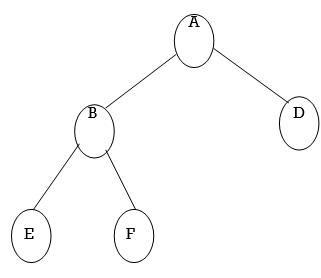
Fig. Binary Tree
To represent this tree, we need an array of size 23+1 - 1 = 15
The tree is represented as follows:
1. The root is stored in BinaryTree[1].
2. For node BinaryTree[n], the left child is stored in BinaryTree[2*n], and the right child is stored in BinaryTree[2*n+1]
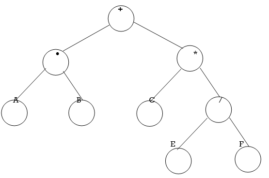
i: 1 2 3 4 5 6 7 8 9 10 11 12 13 14 15
BinaryTree[i]: + - * A B C / E F
Advantages of linear representation:
1. Simplicity.
2. Given the location of the child (say, k), the location of the parent is easy to determine (k / 2).
Disadvantages of linear representation:
1. Additions and deletions of nodes are inefficient, because of the data movements in the array.
2. Space is wasted if the binary tree is not complete. That is, the linear representation is useful if the number of missing nodes is small.
Note that linear representation of a binary tree can be implemented by means of a linked list instead of an array. For example, we can use the Positional Sequence ADT to implement a binary tree in a linear fashion. This way the above mentioned disadvantages of the linear representation will be resolved.
2. Tree representation using Linked List:
Linked list was introduced to reduce the space wastage done by array & also to make easier the insertion and deletion of elements from a list. A binary tree contains nodes of elements where insertion, deletion & searching are frequently done.
Structure of node used to represent tree:
struct node
{
struct node * left;
char data;
struct node * right;
};
The tree shown in 5.10 can be represented using linked list as:
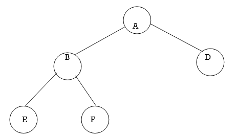
Fig. Representation of Binary Tree using linked list
Traversing a binary tree
Traversal is a process to visit all the nodes of a tree and may print their values too. Because, all nodes are connected via edges (links) we always start from the root (head) node. That is, we cannot randomly access a node in a tree. There are three ways which we use to traverse a tree −
Generally, we traverse a tree to search or locate a given item or key in the tree or to print all the values it contains.
In-order Traversal
In this traversal method, the left subtree is visited first, then the root and later the right sub-tree. We should always remember that every node may represent a subtree itself.
If a binary tree is traversed in-order, the output will produce sorted key values in an ascending order.
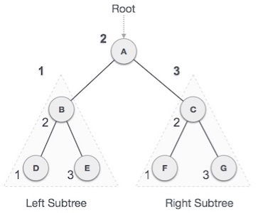
We start from A, and following in-order traversal, we move to its left subtree B. B is also traversed in-order. The process goes on until all the nodes are visited. The output of in order traversal of this tree will be −
D → B → E → A → F → C → G
Algorithm
Until all nodes are traversed −
Step 1 − Recursively traverse left subtree.
Step 2 − Visit root node.
Step 3 − Recursively traverse right subtree.
Pre-order Traversal
In this traversal method, the root node is visited first, then the left subtree and finally the right subtree.
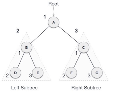
We start from A, and following pre-order traversal, we first visit A itself and then move to its left subtree B. B is also traversed pre-order. The process goes on until all the nodes are visited. The output of pre-order traversal of this tree will be −
A → B → D → E → C → F → G
Algorithm
Until all nodes are traversed −
Step 1 − Visit root node.
Step 2 − Recursively traverse left subtree.
Step 3 − Recursively traverse right subtree.
Post-order Traversal
In this traversal method, the root node is visited last, hence the name. First we traverse the left subtree, then the right subtree and finally the root node.
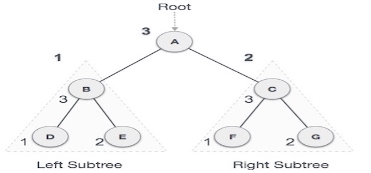
We start from A, and following Post-order traversal, we first visit the left subtree B. B is also traversed post-order. The process goes on until all the nodes are visited. The output of post-order traversal of this tree will be −
D → E → B → F → G → C → A
Algorithm
Until all nodes are traversed −
Step 1 − Recursively traverse left subtree.
Step 2 − Recursively traverse right subtree.
Step 3 − Visit root node.
Implementation in C
#include <stdio.h>
#include <stdlib.h>
struct node {
int data;
struct node *leftChild;
struct node *rightChild;
};
struct node *root = NULL;
void insert(int data) {
struct node *tempNode = (struct node*) malloc(sizeof(struct node));
struct node *current;
struct node *parent;
tempNode->data = data;
tempNode->leftChild = NULL;
tempNode->rightChild = NULL;
//if tree is empty
if(root == NULL) {
root = tempNode;
} else {
current = root;
parent = NULL;
while(1) {
parent = current;
//go to left of the tree
if(data < parent->data) {
current = current->leftChild;
//insert to the left
if(current == NULL) {
parent->leftChild = tempNode;
return;
}
} //go to right of the tree
else {
current = current->rightChild;
//insert to the right
if(current == NULL) {
parent->rightChild = tempNode;
return;
}
}
}
}
}
struct node* search(int data) {
struct node *current = root;
printf("Visiting elements: ");
while(current->data != data) {
if(current != NULL)
printf("%d ",current->data);
//go to left tree
if(current->data > data) {
current = current->leftChild;
}
//else go to right tree
else {
current = current->rightChild;
}
//not found
if(current == NULL) {
return NULL;
}
}
return current;
}
void pre_order_traversal(struct node* root) {
if(root != NULL) {
printf("%d ",root->data);
pre_order_traversal(root->leftChild);
pre_order_traversal(root->rightChild);
}
}
void inorder_traversal(struct node* root) {
if(root != NULL) {
inorder_traversal(root->leftChild);
printf("%d ",root->data);
inorder_traversal(root->rightChild);
}
}
void post_order_traversal(struct node* root) {
if(root != NULL) {
post_order_traversal(root->leftChild);
post_order_traversal(root->rightChild);
printf("%d ", root->data);
}
}
int main() {
int i;
int array[7] = { 27, 14, 35, 10, 19, 31, 42 };
for(i = 0; i < 7; i++)
insert(array[i]);
i = 31;
struct node * temp = search(i);
if(temp != NULL) {
printf("[%d] Element found.", temp->data);
printf("\n");
}else {
printf("[ x ] Element not found (%d).\n", i);
}
i = 15;
temp = search(i);
if(temp != NULL) {
printf("[%d] Element found.", temp->data);
printf("\n");
}else {
printf("[ x ] Element not found (%d).\n", i);
}
printf("\nPreorder traversal: ");
pre_order_traversal(root);
printf("\nInorder traversal: ");
inorder_traversal(root);
printf("\nPost order traversal: ");
post_order_traversal(root);
return 0;
}
If we compile and run the above program, it will produce the following result −
Output
Visiting elements: 27 35 [31] Element found.
Visiting elements: 27 14 19 [ x ] Element not found (15).
Preorder traversal: 27 14 10 19 35 31 42
Inorder traversal: 10 14 19 27 31 35 42
Post order traversal: 10 19 14 31 42 35 27
BST:
We now turn our attention to search tress: Binary Search tress in this chapter and AVL Trees in next chapter. As seen in previous chapter, the array structure provides a very efficient search algorithm, the binary search, but it is inefficient for insertion and deletion algorithms. On the other hand, linked list structure provides efficient insertion and deletion algorithms but it is very inefficient for search algorithm. So what we need is a structure that provides efficient insertion, deletion as well as search algorithms.
Basic Concept:
A Binary Search Tree is a binary tree with the following properties:
1. It may be empty and every node has an identifier.
2. All nodes in left subtree are less than the root.
2. All nodes in right subtree are greater than the root.
4. Each subtree is itself a BST.
Examples of BST:
Valid BSTs:
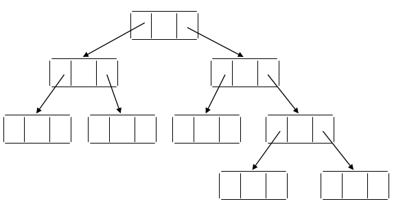
Fig. Examples of Valid BSTs
Invalid BSTs:

Fig. Examples of Invalid BSTs
Examine the BSTs in Fig.4.2. The first tree, Fig.4.2 (a) breaks the second rule: The left node 30 is greater than that of its root node 20. The second tree, Fig.4.2 (b) breaks the third rule: The right node 20 is less than that of its root node 50. The third tree, Fig.4.2 (c) breaks the second rule: The left node 25 is greater than that of its root node 10. It also breaks the third rule: The right node 08 is less than that of its root node 15.
Basic operation
Following are the basic operations of a tree −
Node
Define a node having some data, references to its left and right child nodes.
struct node {
int data;
struct node *leftChild;
struct node *rightChild;
};
Search Operation
Whenever an element is to be searched, start searching from the root node. Then if the data is less than the key value, search for the element in the left subtree. Otherwise, search for the element in the right subtree. Follow the same algorithm for each node.
Algorithm
struct node* search(int data){
struct node *current = root;
printf("Visiting elements: ");
while(current->data != data){
if(current != NULL) {
printf("%d ",current->data);
//go to left tree
if(current->data > data){
current = current->leftChild;
} //else go to right tree
else {
current = current->rightChild;
}
//not found
if(current == NULL){
return NULL;
}
}
}
return current;
}
Insert Operation
Whenever an element is to be inserted, first locate its proper location. Start searching from the root node, then if the data is less than the key value, search for the empty location in the left subtree and insert the data. Otherwise, search for the empty location in the right subtree and insert the data.
Algorithm
void insert(int data) {
struct node *tempNode = (struct node*) malloc(sizeof(struct node));
struct node *current;
struct node *parent;
tempNode->data = data;
tempNode->leftChild = NULL;
tempNode->rightChild = NULL;
//if tree is empty
if(root == NULL) {
root = tempNode;
} else {
current = root;
parent = NULL;
while(1) {
parent = current;
//go to left of the tree
if(data < parent->data) {
current = current->leftChild;
//insert to the left
if(current == NULL) {
parent->leftChild = tempNode;
return;
}
} //go to right of the tree
else {
current = current->rightChild;
//insert to the right
if(current == NULL) {
parent->rightChild = tempNode;
return;
}
}
}
}
}
Threaded Binary Tree
Binary trees, including binary search trees and their variants, can be used to store a set of items in a particular order. For example, a binary search tree assumes data items are ordered and maintain this ordering as part of their insertion and deletion algorithms. One useful operation on such a tree is traversal: visiting the items in the order in which they are stored .A simple recursive traversal algorithm that visits each node of a BST is the following. Assume t is a pointer to a node, or NULL.
Algorithm traverse_tree (root):
Input: a pointer root to a node (or NULL.)
If root = NULL, return.
Else
traverse_tree (left-child (root))
Visit t
traverse_tree (right-child (root))
The problem with this algorithm is that, because of its recursion, it uses stack space proportional to the height of a tree. If the tree is fairly balanced, this amounts to O(log n) space for a tree containing n elements.
One of the solutions to this problem is tree threading.
A threaded binary tree defined as follows:
"A binary tree is threaded by making all right child pointers that would normally be null point to the inorder successor of the node (if it exists), and all left child pointers that would normally be null point to the inorder predecessor of the node."
It is also possible to discover the parent of a node from a threaded binary tree, without explicit use of parent pointers or a stack. This can be useful where stack space is limited, or where a stack of parent pointers is unavailable (for finding the parent pointer via DFS).
Inorder Threaded Binary Tree:
In inorder threaded binary tree, left thread points to the predecessor and right thread points to the successor.
Types Inorder Threaded Binary Tree:
Right Inorder Threaded Binary Tree.
In this type of TBT, only right threads are shown which points to the successor.
Left Inorder Threaded Binary Tree.
In this type of TBT, only left threads are shown which points to the predecessor.
For TBT it is not necessary that the tree must be BST, it can be applied to general tree.
Example: Draw inorder TBT for following data:
10, 8, 1 5, 7, 9, 12, 18
Solution:
Step 1: The general for given data is:
1
8 1
7 9 1 1
Step 2: Write inorder sequence for the above tree:
7, 8, 9, 10, 12, 15, 18
Step 3: Make groups containing three nodes per group like:

Step 4: It means right thread of 7 point to 8 provided that 7 node is not having right link, means right link of 7 is NULL and thread is pointing in bottom-up direction and not in top to bottom .
Left thread of 7 and Right thread of 18 will point to head node.
Step 5: Draw TBT with right and left threads.
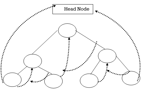
Left Inorder Threaded Binary Tree:

Right Inorder Threaded Binary Tree:

AVL Trees (Adelsion Velski & Landis):
The concept is developed by three persons: Adelsion, Velski and Landis.
Balance Factor:
Balance factor is (Height of left sub tree - Height of right sub tree)
Height Balance Tree:
An empty tree is height balanced. If T is non empty binary tree with TL and TR as left and right sub tress, then T is height balanced if and only if:
TL and TR are height balanced.
HL- HR =1
HL and HR are heights of left and right sub tree.
For ant node in AVL tree Balance factor must be -1 or 0 or 1.
Following rotations are performed on AVL tree if any of the nodes is unbalanced.
1. LL Rotation.
2. LR Rotation.
3. RL Rotation.
4. RR Rotation.
1. LL Rotation:
Count from unbalanced node. First left node becomes the root node.
2. LR Rotation:
Count from unbalanced node. Go for left node and then right node say X. The node X becomes the root node.
3. RL Rotation:
Count from unbalanced node. Go for right node and then left node say X. The node X becomes the root node.
4. RR Rotation:
Count from unbalanced node. First right node becomes the root node.
While inserting data in AVL tree, Follow the property of Binary search tree (left<root<right)
Example: obtain an AVL tree by inserting one integer at a time in following sequence:
150,155,160,115,110,140,120,145,130
SOLUTION:
Step 1: insert 150
150
Balance factor for 150 is: 0 – 0=0
1500
NO ROTATION IS REQUIRED.
Step 2: insert 155
 150-1
150-1
1550
Balance factor for 150 is: 0 – 1= -1
Both nodes are balanced.
NO ROATION IS REQIURED.
STEP 3: INSERT 160.
 150-2
150-2
 155-1
155-1
1600
Balance factor of 150 is -2. So 150 is unbalanced. Some rotation is required to do 150 as balanced node. Start from 150 towards 160.
 150-2 R
155-1 R
1600
We get RR direction. So we have to perform RR rotation.
In RR rotation, Count from unbalanced node. First right node becomes the root node. So here first R is 155. So 155 will become the root.

 1550
1550
1500 1600
Now all nodes are balanced.
STEP 4: INSERT 115.

 1551
1551
 1501 1600
1150
All nodes are balanced. NO ROTATION IS REQUIRED.
STEP 5: INSERT 110

 1552
1552
 1502 1600
 1151
1151
1100
155 and 150 are unbalanced. Whenever two/more nodes are unbalanced, we have to consider the lowermost node first. i.e.150. move from 150 towards the node causing unbalancing (110)


 1552
1552

 L 1502 1600

 L 1151
1100
So we have to perform LL Rotation. In LL rotation, Count from unbalanced node. First Left node becomes the root node. So here first L is 115. So 115 will become the root.


 1551
1551

 1150 1600
1100 1500
Now all nodes are balanced.

 STEP 6: INSERT 140 1552

 115-1 1600
 1100 1501
1400
155 is unbalanced. Count move from 155 towards the node causing unbalancing (140).

 1552
1552
 L
L


 115-1 1600
R
 1100 1501
1400
So we have to perform LR Rotation. In LR rotation, Count from unbalanced node(155). Go for left node and then right node (150). 150 will become root node

 1500
1500


 1150 155-1
1100 1400 1600
Now all nodes are balanced.
STEP 7: INSERT 120

 1501
1501


 115-1 155-1
 1100 1401 1600
1200
Now all nodes are balanced.
STEP 7: INSERT 145

 1501
1501


 115-1 155-1

 1100 1400 1600
1200 1450
Now all nodes are balanced.
STEP 7: INSERT 130

 1502
1502


 115-2 155-1

 1100 1401 1600
 120-1 1450
1300
Two nodes 150 and 115 are unbalanced. First consider 115. Count move from 115 towards the node causing unbalancing (130).

 1502
1502


 115-2 155-1
 R
R

 1100 1401 1600
 L
L
 120-1 1450
1300
So we have to perform RL Rotation. In RL rotation, Count from unbalanced node(115). Go for Right node and then Left node (120). 120 will become root node.


 1501
1501


 1200 155-1


 1150 1400 1600
1100 1300 145
Now all nodes are balanced.


 Thus the tree is balanced.
Reference Books:
1. E Balgurusamy, “Programming in ANSI C”, Tata McGraw-Hill, 3rd Edition.
2. Yedidyah Langsam, Moshe J Augenstein and Aaron M Tenenbaum “Data structures using C and C++” PHI Publications, 2nd Edition.
3. Reema Thareja, “Data Structures using C”, Oxford University Press, 2
nd Edition.
