Unit VI
Graphs
Graph
A graph can be defined as group of vertices and edges that are used to connect these vertices. A graph can be seen as a cyclic tree, where the vertices (Nodes) maintain any complex relationship among them instead of having parent child relationship.
Definition
A graph G can be defined as an ordered set G(V, E) where V(G) represents the set of vertices and E(G) represents the set of edges which are used to connect these vertices.
A Graph G(V, E) with 5 vertices (A, B, C, D, E) and six edges ((A,B), (B,C), (C,E), (E,D), (D,B), (D,A)) is shown in the following figure.

Directed and Undirected Graph
A graph can be directed or undirected. However, in an undirected graph, edges are not associated with the directions with them. An undirected graph is shown in the above figure since its edges are not attached with any of the directions. If an edge exists between vertex A and B then the vertices can be traversed from B to A as well as A to B.
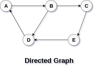
In a directed graph, edges form an ordered pair. Edges represent a specific path from some vertex A to another vertex B. Node A is called initial node while node B is called terminal node.
A directed graph is shown in the following figure.
Graph Terminology
Path
A path can be defined as the sequence of nodes that are followed in order to reach some terminal node V from the initial node U.
Closed Path
A path will be called as closed path if the initial node is same as terminal node. A path will be closed path if V0=VN.
Simple Path
If all the nodes of the graph are distinct with an exception V0=VN, then such path P is called as closed simple path.
Cycle
A cycle can be defined as the path which has no repeated edges or vertices except the first and last vertices.
Connected Graph
A connected graph is the one in which some path exists between every two vertices (u, v) in V. There are no isolated nodes in connected graph.
Complete Graph
A complete graph is the one in which every node is connected with all other nodes. A complete graph contain n(n-1)/2 edges where n is the number of nodes in the graph.
Weighted Graph
In a weighted graph, each edge is assigned with some data such as length or weight. The weight of an edge e can be given as w(e) which must be a positive (+) value indicating the cost of traversing the edge.
Digraph
A digraph is a directed graph in which each edge of the graph is associated with some direction and the traversing can be done only in the specified direction.
Loop
An edge that is associated with the similar end points can be called as Loop.
Adjacent Nodes
If two nodes u and v are connected via an edge e, then the nodes u and v are called as neighbours or adjacent nodes.
Degree of the Node
A degree of a node is the number of edges that are connected with that node. A node with degree 0 is called as isolated node.
In graph theory, a graph representation is a technique to store graph into the memory of computer.
To represent a graph, we just need the set of vertices, and for each vertex the neighbours of the vertex (vertices which is directly connected to it by an edge). If it is a weighted graph, then the weight will be associated with each edge.
There are different ways to optimally represent a graph, depending on the density of its edges, type of operations to be performed and ease of use.
1. Adjacency Matrix
Example
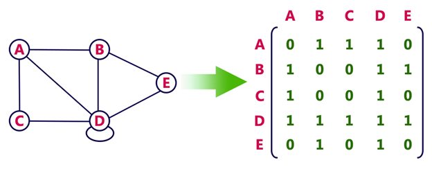
Consider the following undirected graph representation:
Undirected graph representation
Directed graph representation
See the directed graph representation:
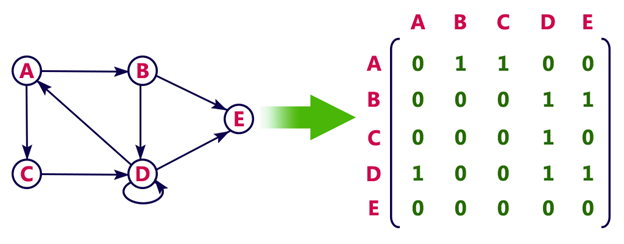
In the above examples, 1 represents an edge from row vertex to column vertex, and 0 represents no edge from row vertex to column vertex.
Undirected weighted graph representation
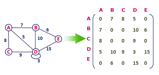
Pros: Representation is easier to implement and follow.
Cons: It takes a lot of space and time to visit all the neighbours of a vertex, we have to traverse all the vertices in the graph, which takes quite some time.
2. Incidence Matrix
In Incidence matrix representation, graph can be represented using a matrix of size:
Total number of vertices by total number of edges.
It means if a graph has 4 vertices and 6 edges, then it can be represented using a matrix of 4X6 class. In this matrix, columns represent edges and rows represent vertices.
This matrix is filled with either 0 or 1 or -1. Where,
Example
Consider the following directed graph representation.

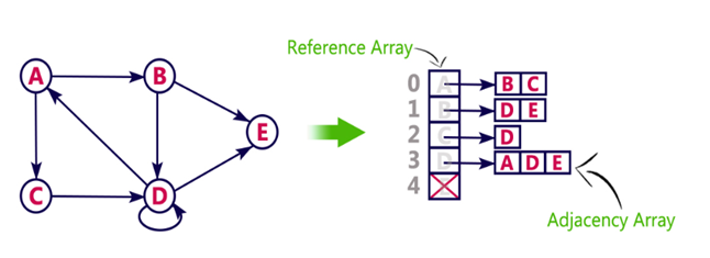
3. Adjacency List
Example
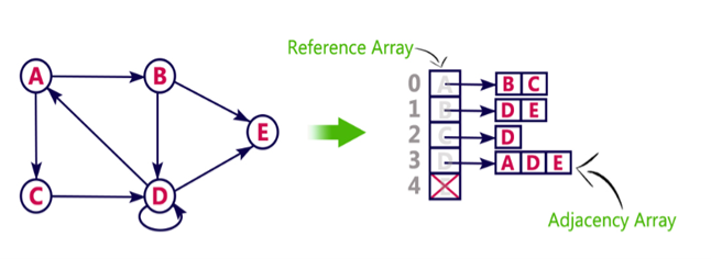
Let's see the following directed graph representation implemented using linked list:

We can also implement this representation using array as follows:
Pros:
Cons:
Graph Operations – Extracting sub graphs
In this section we will discuss about various types of sub graphs we can extract from a given Graph.
Sub graph
Getting a sub graph out of a graph is an interesting operation. A sub graph of a graph G(V,E) can be obtained by the following means:
Points worth noting
We can extract sub graphs for simple graphs, directed graphs, multi edge graphs and all types of graphs.
The Null Graph is always a sub graph of all the graphs. There can be many sub graphs for a graph.
Below is a graph and its sub graphs.

Neighbourhood graph
The neighbourhood graph of a graph G(V,E) only makes sense when we mention it with respect to a given vertex set. For e.g. if V = {1,2,3,4,5} then we can find out the Neighbourhood graph of G(V,E) for vertex set {1}.
So, the neighbourhood graphs contains the vertices 1 and all the edges incident on them and the vertices connected to these edges.
Below is a graph and its neighbourhood graphs as described above.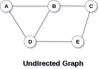
We can also extract neighbourhood graph for a distance more than 1, which means that we do not stop at the first neighbour and also extend it to second, third and more.
Another example for neighbourhood graph up to distance 2 is given below:
Spanning Tree
A spanning tree of a connected graph G(V,E) is a sub graph that is also a tree and connects all vertices in V. For a disconnected graph the spanning tree would be the spanning tree of each component respectively.
There is an interesting set of problems related to finding the minimum spanning tree (which we will be discussing in upcoming posts). There are many algorithms available to solve this problem, for e.g.: Kruskal’s, Prim’s etc. Note that the concept of minimum spanning tree mostly makes sense in case of weighted graphs. If the graph is not weighted, we consider all the weights to be one and any spanning tree becomes the minimum spanning tree.
We can use traversals like Breadth First Scan and Depth First Scan to fight the Spanning Tree. We can find spanning tree for undirected graphs, directed graphs, multi graphs as well.
Below is an example of spanning tree for the given graph.
Graph Operations – Conversions of Graphs
In this section we discuss about converting one graph into another graph. Which means all the graphs can be converted into any of the below forms.
Conversion from Directed Graph to Undirected graph
This is the simplest conversions possible. A directed graph has directions represented by arrows, in this conversion we just remove all the arrows and do not store the direction information. Below is an example of the conversion.
Please note that the graph remains unchanged in terms of its structure. However, we can choose to remove edges if there are multi edges. But it is strictly not required.
Conversion from Undirected Graph to Directed graph
This conversion gives a directed graph given an undirected graph G(V,E). It is the exact reverse of the above. The trick to achieve this is to add one edge for each existing edge in the edge family E. Once the extra edges are added, we just assign opposite direction to each pair of edges between connecting vertices.
Below is a demonstration for the same.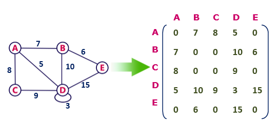
Reversing a graph
Reversing a graph is an operation meant for directed graphs. To reverse a graph we reverse the direction of the edges. The reverse graph has the same vertex set as the original graph. As the edges are reversed, the adjacency matrix for this graph is the Transpose of the adjacency matrix for the original graph (Left to the user to draw and check if this holds true).
Below is the illustration of reversing a graph G(V,E)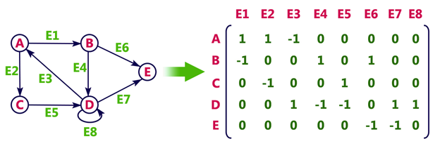
Deriving a Simple graph
The operation is to derive a simple graph out of any given graph. A simple graph by definition must not contain any self loops or multi edges. As we understand that a graph can contain loops and multiple edges, this operation shall remove the loops and multiple edges from the graph G(V,E) to obtain a simple graph.
The adjacency matrix of such a graph will surely have the diagonal elements as zero, because there is no self-loops.
Below is the image to demonstrate this operation.
Graph Operations – Modifications of Graphs
This section talks about some important modifications on a graph. These operations will majorly change the structure of the underlying graph.
Delete Vertex
What happens when we delete a vertex from a given Graph G(V, E)?
We cannot successfully remove a vertex if we do not remove all the edges incident on the vertex. Once we remove the vertex then the adjacency matrix will not contain the row and column for the corresponding vertex.
This operation changes the vertex set and the edge family of the graph.
Below image helps in understanding the removal of vertex.
Contract Vertex
One of the important operations on a graph is contraction. It can be done by contracting two vertices into one. Also, it can be done by contracting an edge, which we will see later in this article.
We cannot contract one vertex, for contraction we need a set of vertices, minimum two. Contraction can only be done when there is an edge between the two vertices. The operation basically removes all the edges between the two vertices.
In the below illustration vertices 1,2 are contracted and 5,6 are also contracted. Please notice the removal of edges between them.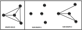
Add & Delete Edge
Adding an edge to a graph can be done by connecting two given vertices.
Deleting an edge can be done by removing the connection between the given vertices. I am not putting any image as it is very trivial operation.
Contracting an Edge
Edge contraction is exactly similar to vertex contraction. It removes the edge from the graph and merges the vertices on which the edge is incident.
Data Structure - Depth First Traversal
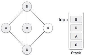
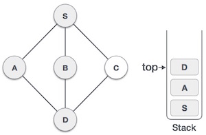
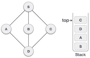
Depth First Search (DFS) algorithm traverses a graph in a depthward motion and uses a stack to remember to get the next vertex to start a search, when a dead end occurs in any iteration.
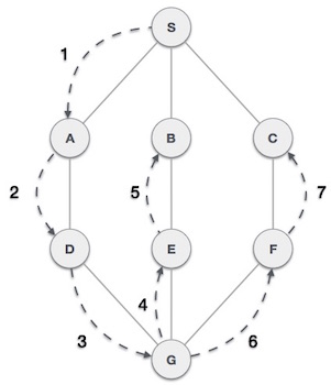
As in the example given above, DFS algorithm traverses from S to A to D to G to E to B first, then to F and lastly to C. It employs the following rules.
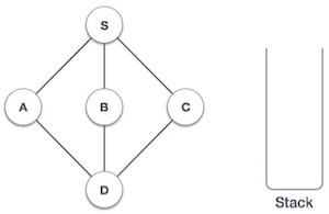
Step | Traversal | Description |
1 |
| Initialize the stack. |
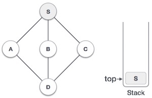
2 |
| Mark S as visited and put it onto the stack. Explore any unvisited adjacent node from S. We have three nodes and we can pick any of them. For this example, we shall take the node in an alphabetical order. |
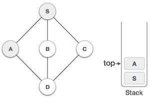
3 |
| Mark A as visited and put it onto the stack. Explore any unvisited adjacent node from A. Both S and D are adjacent to A but we are concerned for unvisited nodes only. |
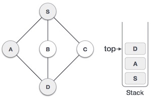
4 |
| Visit D and mark it as visited and put onto the stack. Here, we have B and C nodes, which are adjacent to D and both are unvisited. However, we shall again choose in an alphabetical order. |
5 |
| We choose B, mark it as visited and put onto the stack. Here B does not have any unvisited adjacent node. So, we pop B from the stack. |
6 |
| We check the stack top for return to the previous node and check if it has any unvisited nodes. Here, we find D to be on the top of the stack. |
7 |
| Only unvisited adjacent node is from D is C now. So we visit C, mark it as visited and put it onto the stack. |
As C does not have any unvisited adjacent node so we keep popping the stack until we find a node that has an unvisited adjacent node. In this case, there's none and we keep popping until the stack is empty.
Data Structure - Breadth First Traversal
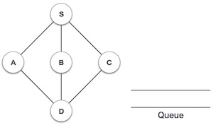
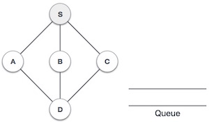
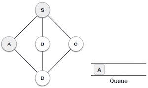
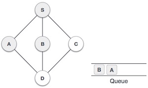
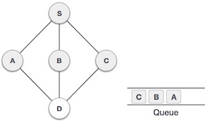
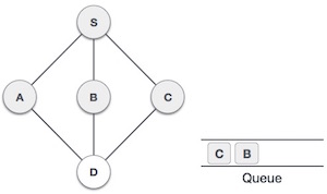
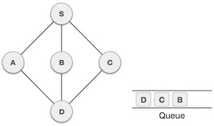
Breadth First Search (BFS) algorithm traverses a graph in a breadth ward motion and uses a queue to remember to get the next vertex to start a search, when a dead end occurs in any iteration.
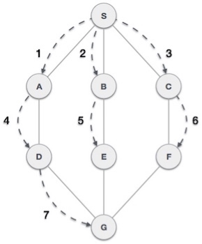
As in the example given above, BFS algorithm traverses from A to B to E to F first then to C and G lastly to D. It employs the following rules.
Step | Traversal | Description |
1 |
| Initialize the queue. |
2 |
| We start from visiting S (starting node), and mark it as visited. |
3 |
| We then see an unvisited adjacent node from S. In this example, we have three nodes but alphabetically we choose A, mark it as visited and enqueue it. |
4 |
| Next, the unvisited adjacent node from S is B. We mark it as visited and enqueue it. |
5 |
| Next, the unvisited adjacent node from S is C. We mark it as visited and enqueue it. |
6 |
| Now, S is left with no unvisited adjacent nodes. So, we dequeue and find A. |
7 |
| From A we have D as unvisited adjacent node. We mark it as visited and enqueue it. |
At this stage, we are left with no unmarked (unvisited) nodes. But as per the algorithm we keep on dequeuing in order to get all unvisited nodes. When the queue gets emptied, the program is over.
Spanning Tree
A spanning tree is a subset of Graph G, which has all the vertices covered with minimum possible number of edges. Hence, a spanning tree does not have cycles and it cannot be disconnected.
By this definition, we can draw a conclusion that every connected and undirected Graph G has at least one spanning tree. A disconnected graph does not have any spanning tree, as it cannot be spanned to all its vertices.
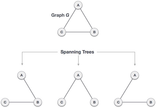
We found three spanning trees off one complete graph. A complete undirected graph can have maximum nn-2 number of spanning trees, where n is the number of nodes. In the above addressed example, n is 3, hence 33−2 = 3 spanning trees are possible.
General Properties of Spanning Tree
We now understand that one graph can have more than one spanning tree. Following are a few properties of the spanning tree connected to graph G −
Mathematical Properties of Spanning Tree
Thus, we can conclude that spanning trees are a subset of connected Graph G and disconnected graphs do not have spanning tree.
Application of Spanning Tree
Spanning tree is basically used to find a minimum path to connect all nodes in a graph. Common application of spanning trees is −
Let us understand this through a small example. Consider, city network as a huge graph and now plans to deploy telephone lines in such a way that in minimum lines we can connect to all city nodes. This is where the spanning tree comes into picture.
Minimum Spanning Tree (MST)
In a weighted graph, a minimum spanning tree is a spanning tree that has minimum weight than all other spanning trees of the same graph. In real-world situations, this weight can be measured as distance, congestion, traffic load or any arbitrary value denoted to the edges.
Kruskal's Spanning Tree
Kruskal's algorithm to find the minimum cost spanning tree uses the greedy approach. This algorithm treats the graph as a forest and every node it has as an individual tree. A tree connects to another only and only if, it has the least cost among all available options and does not violate MST properties.
To understand Kruskal's algorithm let us consider the following example −
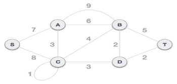
Step 1 - Remove all loops and Parallel Edges
Remove all loops and parallel edges from the given graph.
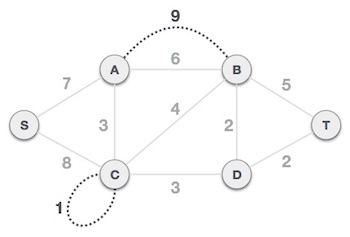
In case of parallel edges, keep the one which has the least cost associated and remove all others.
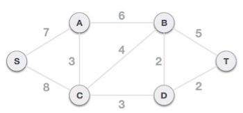
Step 2 - Arrange all edges in their increasing order of weight
The next step is to create a set of edges and weight, and arrange them in an ascending order of weightage (cost).

Step 3 - Add the edge which has the least weightage
Now we start adding edges to the graph beginning from the one which has the least weight. Throughout, we shall keep checking that the spanning properties remain intact. In case, by adding one edge, the spanning tree property does not hold then we shall consider not to include the edge in the graph.
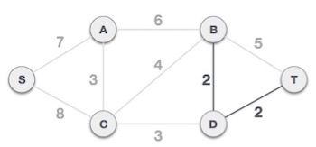
The least cost is 2 and edges involved are B,D and D,T. We add them. Adding them does not violate spanning tree properties, so we continue to our next edge selection.
Next cost is 3, and associated edges are A,C and C,D. We add them again −
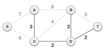
Next cost in the table is 4, and we observe that adding it will create a circuit in the graph. −
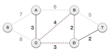
We ignore it. In the process we shall ignore/avoid all edges that create a circuit.
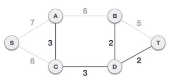
We observe that edges with cost 5 and 6 also create circuits. We ignore them and move on.
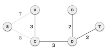
Now we are left with only one node to be added. Between the two least cost edges available 7 and 8, we shall add the edge with cost 7.
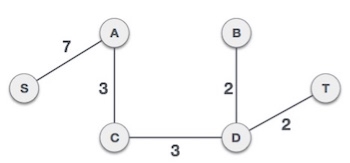
By adding edge S,A we have included all the nodes of the graph and we now have minimum cost spanning tree.
Prim's Spanning Tree
Prim's algorithm to find minimum cost spanning tree (as Kruskal's algorithm) uses the greedy approach. Prim's algorithm shares a similarity with the shortest path first algorithms.
Prim's algorithm, in contrast with Kruskal's algorithm, treats the nodes as a single tree and keeps on adding new nodes to the spanning tree from the given graph.
To contrast with Kruskal's algorithm and to understand Prim's algorithm better, we shall use the same example −
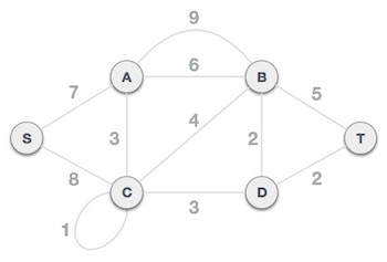
Step 1 - Remove all loops and parallel edges

Remove all loops and parallel edges from the given graph. In case of parallel edges, keep the one which has the least cost associated and remove all others.
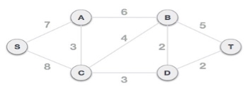
Step 2 - Choose any arbitrary node as root node
In this case, we choose S node as the root node of Prim's spanning tree. This node is arbitrarily chosen, so any node can be the root node. One may wonder why any video can be a root node. So the answer is, in the spanning tree all the nodes of a graph are included and because it is connected then there must be at least one edge, which will join it to the rest of the tree.
Step 3 - Check outgoing edges and select the one with less cost
After choosing the root node S, we see that S,A and S,C are two edges with weight 7 and 8, respectively. We choose the edge S,A as it is lesser than the other.
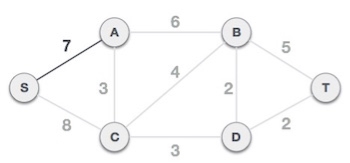
Now, the tree S-7-A is treated as one node and we check for all edges going out from it. We select the one which has the lowest cost and include it in the tree.
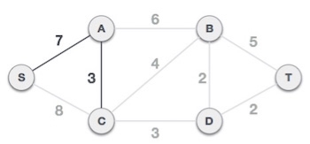
After this step, S-7-A-3-C tree is formed. Now we'll again treat it as a node and will check all the edges again. However, we will choose only the least cost edge. In this case, C-3-D is the new edge, which is less than other edges' cost 8, 6, 4, etc.
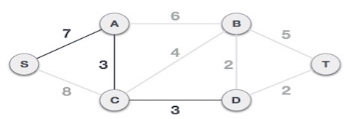
After adding node D to the spanning tree, we now have two edges going out of it having the same cost, i.e. D-2-T and D-2-B. Thus, we can add either one. But the next step will again yield edge 2 as the least cost. Hence, we are showing a spanning tree with both edges included.
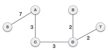
We may find that the output spanning tree of the same graph using two different algorithms is same.
Dijkstra's Algorithm
Dijkstra's algorithm has many variants but the most common one is to find the shortest paths from the source vertex to all other vertices in the graph.
Algorithm Steps:
with the new distance to the priority queue.
Implementation:
Assume the source vertex =
.
#define SIZE 100000 + 1
vector < pair < int , int > > v [SIZE]; // each vertex has all the connected vertices with the edges weights
int dist [SIZE];
bool vis [SIZE];
void dijkstra(){
// set the vertices distances as infinity
memset(vis, false , sizeof vis); // set all vertex as unvisited
dist[1] = 0;
multiset < pair < int , int > > s; // multiset do the job as a min-priority queue
s.insert({0 , 1}); // insert the source node with distance = 0
while(!s.empty()){
pair <int , int> p = *s.begin(); // pop the vertex with the minimum distance
s.erase(s.begin());
int x = p.s; int wei = p.f;
if( vis[x] ) continue; // check if the popped vertex is visited before
vis[x] = true;
for(int i = 0; i < v[x].size(); i++){
int e = v[x][i].f; int w = v[x][i].s;
if(dist[x] + w < dist[e] ){ // check if the next vertex distance could be minimized
dist[e] = dist[x] + w;
s.insert({dist[e], e} ); // insert the next vertex with the updated distance
}
}
}
}
Time Complexity of Dijkstra's Algorithm is
but with min-priority queue it drops down to
.
However, if we have to find the shortest path between all pairs of vertices, both of the above methods would be expensive in terms of time. Discussed below is another algorithm designed for this case.
Dijkstra’s Algorithm
Dijkstra’s algorithm solves the single-source shortest-paths problem on a directed weighted graph G = (V, E), where all the edges are non-negative (i.e., w(u, v) ≥ 0 for each edge (u, v) Є E).
In the following algorithm, we will use one function Extract-Min(), which extracts the node with the smallest key.
Algorithm: Dijkstra’s-Algorithm (G, w, s)
for each vertex v Є G.V
v.d := ∞
v.∏ := NIL
s.d := 0
S := Ф
Q := G.V
while Q ≠ Ф
u := Extract-Min (Q)
S := S U {u}
for each vertex v Є G.adj[u]
if v.d > u.d + w(u, v)
v.d := u.d + w(u, v)
v.∏ := u
Analysis
The complexity of this algorithm is fully dependent on the implementation of Extract-Min function. If extract min function is implemented using linear search, the complexity of this algorithm is O(V2 + E).
In this algorithm, if we use min-heap on which Extract-Min() function works to return the node from Q with the smallest key, the complexity of this algorithm can be reduced further.
Example
Let us consider vertex 1 and 9 as the start and destination vertex respectively. Initially, all the vertices except the start vertex are marked by ∞ and the start vertex is marked by 0.
Vertex | Initial | Step1 V1 | Step2 V3 | Step3 V2 | Step4 V4 | Step5 V5 | Step6 V7 | Step7 V8 | Step8 V6 |
1 | 0 | 0 | 0 | 0 | 0 | 0 | 0 | 0 | 0 |
2 | ∞ | 5 | 4 | 4 | 4 | 4 | 4 | 4 | 4 |
3 | ∞ | 2 | 2 | 2 | 2 | 2 | 2 | 2 | 2 |
4 | ∞ | ∞ | ∞ | 7 | 7 | 7 | 7 | 7 | 7 |
5 | ∞ | ∞ | ∞ | 11 | 9 | 9 | 9 | 9 | 9 |
6 | ∞ | ∞ | ∞ | ∞ | ∞ | 17 | 17 | 16 | 16 |
7 | ∞ | ∞ | 11 | 11 | 11 | 11 | 11 | 11 | 11 |
8 | ∞ | ∞ | ∞ | ∞ | ∞ | 16 | 13 | 13 | 13 |
9 | ∞ | ∞ | ∞ | ∞ | ∞ | ∞ | ∞ | ∞ | 20 |
Hence, the minimum distance of vertex 9 from vertex 1 is 20. And the path is
1→ 3→ 7→ 8→ 6→ 9
This path is determined based on predecessor information.
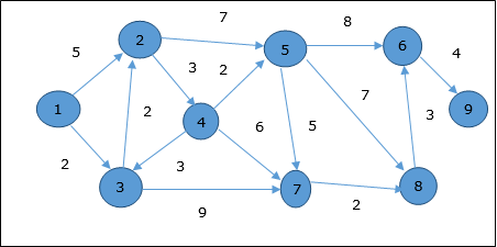
Bellman Ford Algorithm
This algorithm solves the single source shortest path problem of a directed graph G = (V, E) in which the edge weights may be negative. Moreover, this algorithm can be applied to find the shortest path, if there does not exist any negative weighted cycle.
Algorithm: Bellman-Ford-Algorithm (G, w, s)
for each vertex v Є G.V
v.d := ∞
v.∏ := NIL
s.d := 0
for i = 1 to |G.V| - 1
for each edge (u, v) Є G.E
if v.d > u.d + w(u, v)
v.d := u.d +w(u, v)
v.∏ := u
for each edge (u, v) Є G.E
if v.d > u.d + w(u, v)
return FALSE
return TRUE
Analysis
The first for loop is used for initialization, which runs in O(V) times. The next for loop runs |V - 1| passes over the edges, which takes O(E) times.
Hence, Bellman-Ford algorithm runs in O(V, E) time.
Example
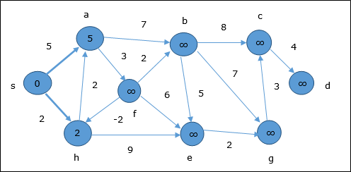
The following example shows how Bellman-Ford algorithm works step by step. This graph has a negative edge but does not have any negative cycle, hence the problem can be solved using this technique.
At the time of initialization, all the vertices except the source are marked by ∞ and the source is marked by 0.
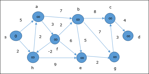
In the first step, all the vertices which are reachable from the source are updated by minimum cost. Hence, vertices a and h are updated.
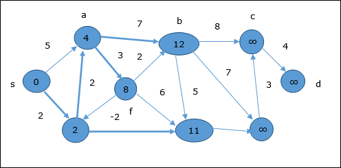
In the next step, vertices a, b, f and e are updated.
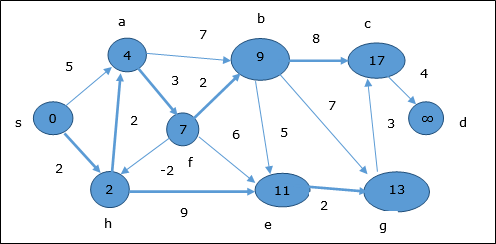
Following the same logic, in this step vertices b, f, c and g are updated.
Here, vertices c and d are updated.
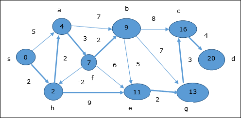
Hence, the minimum distance between vertex s and vertex d is 20.
Based on the predecessor information, the path is s→ h→ e→ g→ c→ d
Reference Books:
1. E Balgurusamy, “Programming in ANSI C”, Tata McGraw-Hill, 3rd Edition.
2. Yedidyah Langsam, Moshe J Augenstein and Aaron M Tenenbaum “Data structures using C and C++” PHI Publications, 2nd Edition.
3. Reema Thareja, “Data Structures using C”, Oxford University Press, 2
nd Edition.
