Unit - 1

Introduction to DBMS

1.1 Introduction to Database Management Systems

Database

The database is a set of interrelated data used to efficiently retrieve, insert and remove data. It is also used in the form of a table, schema, views, and reports to organize the data, etc.

You can conveniently retrieve, attach, and delete information using the database.

Database management system (DBMS)

A DBMS is a programme that enables database creation, specification and manipulation, allowing users to easily store, process and analyse information.

DBMS provides one with an interface or a tool to conduct different operations, such as building databases, storing data in them, updating data, creating database tables, and much more.

The DBMS also provides databases with privacy and security. In the case of multiple users, it also ensures data consistency.

Some Example of DBMS:

●      MySQL

●      Oracle

●      SQL Server

●      IBM DB2

Advantages of DBMS

●      Controls database redundancy: It can control data redundancy because it stores all the data in one single database file and that recorded data is placed in the database.

●      Data sharing: In DBMS, the authorized users of an organization can share the data among multiple users.

●      Easily Maintenance: It can be easily maintainable due to the centralized nature of the database system.

●      Reduce time: It reduces development time and maintenance need.

●      Backup: It provides backup and recovery subsystems which create automatic backup of data from hardware and software failures and restores the data if required.

●      multiple user interface: It provides different types of user interfaces like graphical user interfaces, application program interfaces

Disadvantages of DBMS

●      Cost of Hardware and Software: It requires a high speed of data processor and large memory size to run DBMS software.

●      Size: It occupies a large space of disks and large memory to run them efficiently.

●      Complexity: Database system creates additional complexity and requirements.

●      Higher impact of failure: Failure is highly impacted the database because in most of the organization, all the data stored in a single database and if the database is damaged due to electric failure or database corruption then the data may be lost forever.

1.2 Purpose of Database Systems

It is a set of tools that allows a user to construct and manage databases. In other words, it is general-purpose software that enables users to define, construct, and manipulate databases for a variety of applications.

Database systems are made to handle massive amounts of data. Data management entails both the creation of structures for storing data and the provision of methods for manipulating data. Furthermore, despite system crashes or efforts at illegal access, the database system must preserve the security of the information stored. If data is to be shared across multiple users, the system must avoid any unexpected outcomes.

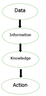
Fig 1: Process of transforming data

The figure above depicts the process of transforming data into information, knowledge, and action in a database management system.

The file system was used as the foundation for the database applications.

The goal of a database management system (DBMS) is to transform the following:

1. Data into information.

2. Information into knowledge.

3. Knowledge of the action.

Uses of DBMS

The main uses of DBMS are as follows −

●      Data independence and efficient access of data.

●      Application Development time reduces.

●      Security and data integrity.

●      Uniform data administration.

●      Concurrent access and recovery from crashes.

Characteristics of DBMS

●      It stores and manages information in a digital repository hosted on a server.

●      It can provide a logical and transparent picture of the data manipulation process.

●      Automatic backup and recovery mechanisms are included in the DBMS.

●      It has ACID qualities, which keep data healthy in the event of a failure.

●      It has the ability to simplify complex data relationships.

●      It's utilized to help with data manipulation and processing.

●      It is used to ensure data security.

●      It can examine the database from several perspectives depending on the user's needs.

1.3 Database-System Applications

Data is a collection of linked facts and statistics that may be processed to provide information, and a database is a collection of related data.

The majority of data is made up of observable facts. Data assists in the creation of fact-based content. For example, if we have data on all students' grades, we can draw conclusions about top performers and average grades.

A database management system maintains data in such a way that retrieving, manipulating, and producing information becomes easy. The following are some of the most notable DBMS properties and applications.

●      ACID Properties - Atomicity, Consistency, Isolation, and Durability are all concepts that DBMS adheres to (normally shortened as ACID). These principles are used to manipulate data in a database through transactions. In multi-transactional situations and in the event of failure, ACID features assist the database stay healthy.

●      Multiuser and Concurrent Access - The DBMS enables a multi-user environment, allowing multiple users to access and manipulate data at the same time. Although there are limitations on transactions when many users attempt to handle the same data item, the users are never aware of them.

●      Multiple views - For different users, DBMS provides multiple perspectives. A user in the Sales department will see the database in a different way than someone in the Production department. This feature allows users to get a focused view of the database based on their specific needs.

●      Security - Multiple views, for example, provide some security by preventing users from accessing data belonging to other users or departments. When entering data into a database and retrieving it later, DBMS provides mechanisms to set limitations. Multiple users can have distinct perspectives with various functionalities thanks to DBMS's many different levels of security features. A user in the Sales department, for example, cannot see data from the Purchase department. It can also be controlled how much data from the Sales department is displayed to the user. Because DBMSs are not kept on disk like traditional file systems, it is extremely difficult for criminals to crack the coding.

1.4 Data Abstraction and Database System Structure

●      A major objective of database systems is to provide users with an abstract view of the data.

●      The system hides details of how the data is stored and maintained.

●      Database systems has to provide an efficient mechanism for data retrieval.

●      Efficiency leads to the design of complex data structure for representation of data in databases.

●      This complexity must be hidden from users.

●      This can be done by providing several levels of abstractions.

●      In the Three Schema Architecture, three levels of abstraction have been created. 

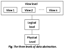
Fig 2: Data abstraction

These are: -

●      Logical level: This is the middle stage of the architecture of 3-level data abstraction. This explains what information is contained in the database.

●      View level: Highest data abstraction standard. This level defines the relationship between users and the database system.

●      Physical level: This is the lowest data abstraction level. This explains how the data in the database is actually stored. At this step, you can get the complex information of the data structure.

Database System Structure

The architecture of a database management system influences its design. When dealing with a large number of PCs, web servers, database servers, and other networked elements, the same client/server architecture is used.

A client/server architecture is made up of several PCs and a workstation that are all linked by a network.

The design of a database management system is determined by how users link to the database in order to complete their requests.

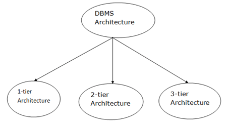
Fig 1: Types of architecture

A single tier or multi-tier database architecture can be seen. However, database design can be divided into two categories: 2-tier architecture and 3-tier architecture.

1-tier Architecture:

The database is directly accessible to the user in this architecture. It means that the user can sit on the DBMS and use it directly. Any modifications made here will be applied directly to the database. It does not provide end users with a useful tool.

For the creation of local applications, a 1-tier architecture is used, in which programmers can interact directly with the database for fast responses.

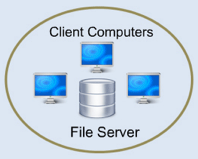
Fig4: 1-tier architecture

2-tier Architecture:

The 2-tier architecture is similar to the basic client-server architecture. Client-side applications can interact directly with the database on the server side in a two-tier architecture. APIs such as ODBC and JDBC are used for this interaction.

The client-side runs the user interfaces and application programs. The server side is in charge of providing features such as query processing and transaction management. The client-side application creates a link with the server side in order to communicate with the DBMS.

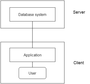
Fig 5: 2-tier architecture

3-tier Architecture:

Between the client and the server is another layer in the 3-tier architecture. The client cannot communicate directly with the server in this architecture. The client-side program communicates with an application server, which in turn communicates with the database system.

Beyond the application server, the end user is unaware of the database's presence. Aside from the submission, the database has no knowledge about any other users.

In the case of a wide web application, the 3-tier architecture is used.

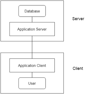
Fig 6: 3-tier architecture

Key takeaway:

1. The system hides details of how the data is stored and maintained.
2. Complexity must be hidden from users.

1.5 Relational Model: Structure of relational databases, Domains, Relations

The primary data model is the Relational Data Model, which is commonly used for data storage and processing around the world. This model is simple and has all the features and functionality needed to process data with efficiency in storage.

The relational model can be interpreted as a table with rows and columns. Each row is called a tuple. There's a name or attribute for each table in the column.

Structure

A relational database is made up of several tables.

- Each table is given its own name.

– There are several rows in each table.

– Each row is a collection of data that are, by definition, related to one another in some way; these values correspond to the table's attributes or columns.

– Each table attribute has a set of authorized values for that attribute; this set of permitted values is the attribute's domain.

Basic concept:

Attributes and Domains

Relations

Example: STUDENT Relation

●      In the given table, NAME, ROLL_NO, PHONE_NO, ADDRESS, and AGE are the attributes.

●      The instance of schema STUDENT has 5 tuples.

●      t3 = <Laxman, 33289, 8583287182, Gurugram, 20>

1.6 Relational algebra – fundamental operators and syntax, relational algebra queries

Relational Algebra is procedural query language. It takes Relation as input and generates relation as output. Relational algebra mainly provides theoretical foundation for relational databases and SQL.

Basic Operations which can be performed using relational algebra are:

1. Projection

2. Selection

3. Join

4. Union

5. Set Difference

6. Intersection

7. Cartesian product

8. Rename

Consider following relation R (A, B, C)

1. Projection (π):

This operation is used to select particular columns from the relation.

Π(AB) R:

It will select A and B column from the relation R. It produces the output like:

Project operation automatically removes duplicates from the resultant set.

Example

∏subject, author (Books)

Selects and projects columns named as subject and author from the relation Books.

2.     Selection (σ):

This operation is used to select particular tuples from the relation.

σ(C<4) R:

It will select the tuples which have value of c less than 4.

But select operation is used to only select the required tuples from the relation. To display those tuples on screen, select operation must be combined with project operation.

Π (σ (C<4) R) will produce the result like:

Example

σ sales > 50000 (Customers)

Output – Selects tuples from Customers where sales is greater than 5000

3.     Join 

A Cartesian product followed by a selection criterion is basically a joint process.

Operation of join, denoted by ⋈

The JOIN operation often allows tuples from different relationships to join different tuples

Types of JOIN:

Various forms of join operation are:

Inner Joins:

●      Theta join

●      EQUI join

●      Natural join

Outer join:

●      Left Outer Join

●      Right Outer Join

●      Full Outer Join

4.     Union

Union operation in relational algebra is the same as union operation in set theory, only the restriction is that both relations must have the same set of attributes for a union of two relationships.

Syntax:  table_name1 ∪ table_name2

For instance, if we have two tables with Regular Class and Extra Class, both have a student column to save the student name, then,

∏Student(RegularClass) ∪ ∏Student(ExtraClass)

The above operation will send us the names of students who attend both normal and extra classes, reducing repetition.

5.     Set difference

Set Difference in relational algebra is the same operation of set difference as in set theory, with the limitation that the same set of attributes can have both relationships.

Syntax: A - B

Where the A and B relationships.

For instance, if we want to find the names of students who attend the regular class, but not the extra class, then we can use the following procedure:

∏Student(RegularClass) - ∏Student(ExtraClass)

Example

∏ author (Books) − ∏ author (Articles)

Output − Provides the name of authors who have written books but not articles.

6.     Intersection

The symbol ∩ is the definition of an intersection.

A ∩ B

Defines a relationship consisting of a set of all the tuples in both A and B. A and B must be union-compatible, however.

7.     Cartesian product

This is used to merge information into one from two separate relationships(tables) and to fetch information from the merged relationship.

Syntax: A X B

For example, if we want to find the morning Regular Class and Extra Class data, then we can use the following operation:

σtime = 'morning' (RegularClass X ExtraClass)

Both RegularClass and ExtraClass should have the attribute time for the above query to operate.

8.     Rename

Rename is a unified operation that is used to rename relationship attributes.

ρ (a/b)R renames the 'b' component of the partnership to 'a'.

Syntax: ρ(RelationNew, RelationOld)

Key takeaway:

1. Relational Algebra is procedural query language.
2. It takes Relation as input and generates relation as output.
3. Data stored in a database can be retrieved using query.

1.7 Tuple relational calculus

●      To select the tuples in a relationship, the tuple relational calculus is defined. The filtering variable in TRC uses relationship tuples.

●      You may have one or more tuples as a consequence of the partnership.

Notation: {T | P (T)} or {T | Condition (T)}

Where,

T - resulting tuple

P (T) - condition used to fetch T.

Example 1:

{T.name | Author(T) AND T.article = 'database’} 

Output:

Select tuples from the AUTHOR relationship in this question. It returns a 'name' tuple from the author who wrote a 'database' post.

TRC (tuple relation calculus) can be quantified. We may use existential (∃) and universal quantifiers (∀) in TRC.

Example 2:

{R| ∃T ∈ Authors(T.article='database' AND R.name=T.name)} 

Output: This question is going to generate the same result as the previous one.

1.8 Entity-Relationship model: Basic Concepts, Entity Set, Relationship Sets and Weak Entity Sets

●      The Entity-Relationship model (ER model) is a type of entity-relationship model. It's a data model at a high level. The data elements and relationships for a given system are described using this model.

●      It creates a database's conceptual architecture. It also creates a very convenient and easy-to-design data view.

●      The database structure is depicted as a diagram called an entity-relationship diagram in ER modeling.

Let's say we're creating a database for a school. The student will be an object in this database, with attributes such as address, name, id, age, and so on. There will be a relationship between the address and another entity with attributes such as city, street name, pin code, and so on.

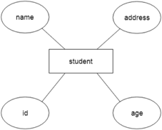
Fig 7: Example of ER

Component of ER model -

The following components are composed of an ER Diagram:

1. Entity
2. Attributes
3. Relationships

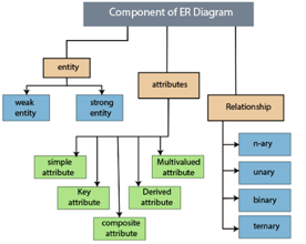
Fig 8: Component of ER model

Entity

The object, location, person, or event that stores data in the database may be an entity. In an object-relationship diagram, a rectangle represents an entity.

Examples of an individual include a student, course, boss, employee, patient, etc.

Fig 9: Entity

Entity type:

A list or a set of entities having certain common attributes is an entity type. In a database, a name and a list of attributes define each type of entity.

Entity set:

It is a set (or collection) of entities of the same kind that share attributes or related properties.

For example, it is possible to describe the category of individuals who are lecturers at a university as an entity-set lecturer. Similarly, the collection of students of the organization could represent the community of all university students.

Attribute

In an Entity-Relationship Model, an attribute defines an entity's properties or characteristics. It is represented in the ER diagram by an oval or ellipse shape. Each oval shape represents one attribute and is directly linked to the person that is in the shape of the rectangle.

For instance, the attributes defining the Employee form of entity are employee id, employee name, gender, employee age, salary, and mobile no.

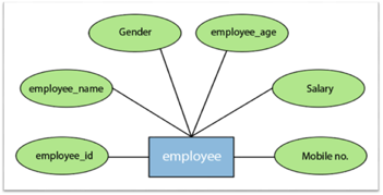
Fig 10: Different attributes of employee

In the ER model, the following categories can be defined by an attribute:

1.Simple attribute:

A simple attribute is called an attribute which contains an atomic value and cannot be divided further. The gender and salary of a worker, for instance, is also depicted by an oval.

2. Key attribute:

A key attribute is called an attribute that can uniquely identify an entity in an entity set. It represents a primary key in the ER diagram. In an Entity Relationship diagram, the key attribute is denoted by an oval with an underlying line. For example, for each employee, the employee id would be unique.

3. Composite attribute:

An attribute that is a combination of two or more basic attributes is called a composite attribute. It is defined by an ellipse in an Entity-Relationship diagram, and that ellipse consists of other ellipses. For example, an employee entity type's name attribute consists of first name, second name, and last name.

4.Derived attribute:

A derived attribute is considered an attribute which can be derived from other attributes. In an entity-relationship diagram, a dashed oval shape is used to represent these attributes. Employee age is, for example, a derived attribute since it varies over time and can be derived from another DOB attribute (Date of birth).

5.Multivalued attributes:

An attribute which for a given entity contains more than one value. For instance, there may be more than one mobile number and email address for an employee.

Entity Set

Student

An entity set is a collection of entities that are similar in nature. It may contain entities with attribute values that are comparable. Properties, often known as attributes, are used to represent entities. Each attribute has its own set of values. A student object, for example, may have properties such as name, age, and class.

Fig 11: Example of entity

Entities as an example:

Some departments may exist at a university. All of these departments employ a variety of lecturers and provide a variety of programs.

Each program is made up of a few courses. Students enroll in several courses after registering for a certain program. Each course is taught by a lecturer from a certain department, and each lecturer teaches a different set of students.

Relationship Sets

In the Entity-Relation Model, a relationship is used to define the relationship between two or more entities. In the ER diagram, it is illustrated by a diamond shape.

For example, in college student studies, employees work in a department. Here, the links are 'research in' and 'works in'.

Degree of Relationship

A partnership is called the degree of a relationship in which a variety of different individuals participate.

Degree of relationship can be categorized into the following types:

1. Unary Relationship:

A relationship in which a single group of individuals is involved is referred to as a unary relationship. For instance, in a company, an employee manages or supervises another employee.

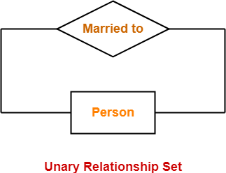
Fig 12: Unary relationship set

2. Binary Relationship: When a relationship includes two people, it is considered a binary relationship.

Fig 13: Binary relationship set

3. Ternary Relationship: When a relationship contains three individual sets, a ternary relationship is called.

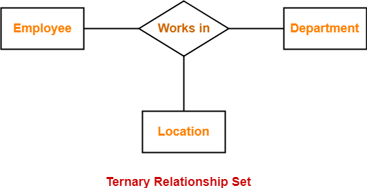
Fig 14: Ternary relationship set

4. N-nary Relationship:

If a relationship includes more than three entity sets, an n-ary relationship is named.

Weak Entity Sets 

Although an entity type should contain a key attribute that uniquely identifies each entity in the entity collection, some entity types do not have a key attribute. Weak Entity is the name given to this type of entity.

Weak entity sets are those with insufficient qualities to generate a primary key, while strong entity sets are those with a primary key.

Because weak entities lack a primary key, they can't be identified on their own and must rely on another object (known as owner entity). In their identifying link with the owner identity, the weak entities face a whole participation constraint (existence dependency). Partially keyed entity types exist. Partial Keys are a set of properties that can be used to distinguish and identify the tuples of weak entities.

The existence of a weak entity is contingent on the existence of a strong entity. Weak entity, like a strong entity, does not have a primary key, but it does have a partial discriminator key. The double rectangle represents a weak entity. A double diamond represents the relationship between two strong and weak entities.

In the ER Diagram, weak entities are represented by a double rectangular box, while identifying linkages are represented by a double diamond. Dotted lines are used to express partial key attributes.

Fig 15: Weak entity set

Key takeaway:

1. The object, location, person, or event that stores data in the database may be an entity.
2. In an Entity-Relationship Model, an attribute defines an entity's properties or characteristics.
3. Attributes are represented in the ER diagram by an oval or ellipse shape.
4. In the Entity-Relation Model, a relationship is used to define the relationship between two or more entities.

1.9 Mapping Cardinalities

●      A mapping constraint is a data constraint representing the number of entities to which a relationship set can relate to another entity.

●      It is most useful to define relationship sets involving more than two sets of individuals.

●      There are four possible mapping cardinalities for the binary relationship set R on an entity set A and B. They are as follows

1. One to one (1:1)
2. One to many (1:M)
3. Many to many (M:M)

One to one: As we have seen in the example above, only one instance of an entity is mapped to one instance of another entity. Consider the Department's HOD. Just one HOD in one department exists. That is, the relationship between the HOD agency and the Department is 1:1.

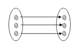
Fig 16: One to one mapping

One to many: As we can guess now, there is one instance of an entity linked to many instances of another entity between one and several relationships. In his department, one manager oversees several employees.

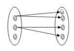
Fig 17: One to many mapping

Many to many: This is a relationship where multiple entity instances are linked to multiple entity instances.

Fig 18: Many to many mapping

Key takeaway:

●      It is most useful to define relationship sets involving more than two sets of individuals.

●      There are four possible mapping cardinalities for the binary relationship.

1.10 Keys

Keys are the entity's attributes, which define the entity's record uniquely.

Several types of keys exist.

These are listed underneath:

●      Composite key

A composite key consists of two attributes or more, but it must be minimal.

●      Candidate key

A candidate key is a key that is simple or composite and special and minimal. It is special since no two rows can have the same value at any time in a table. It is minimal since, in order to achieve uniqueness, every column is required.

●      Super key

The Super Key is one or more of the entity's attributes that uniquely define the database record.

●      Primary key

The primary key is a candidate key that the database designer chooses to be used as an identification mechanism for the entire set of entities. In a table, it must uniquely classify tuples and not be null.

In the ER model, the primary key is indicated by underlining the attribute.

●      To uniquely recognize tuples in a table, the designer selects a candidate key. It must not be empty.

●      A key is selected by the database builder to be used by the entire entity collection as an authentication mechanism. This is regarded as the primary key. In the ER model, this key is indicated by underlining the attribute.

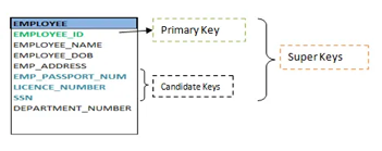
Fig 19: Shows different keys

●      Alternate key

Alternate keys are all candidate keys not chosen as the primary key.

●      Foreign key

A foreign key (FK) is an attribute in a table that, in another table, references the primary key OR it may be null. The same data type must be used for both international and primary keys.

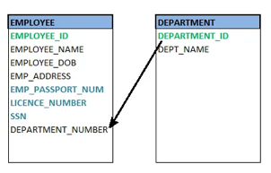
Fig 20: Foreign key

●      Secondary key

A secondary key is an attribute used exclusively (can be composite) for retrieval purposes, such as: phone and last name.

Key takeaway:

●      Keys are the entity's attributes, which define the entity's record uniquely.

●      A candidate key is a key that is simple or composite and special and minimal.

●      Primary key, uniquely recognize tuples in a table, the designer selects a candidate key. It must not be empty.

1.11 E-R diagrams

●      The logical structure of a database can be expressed by an E-R diagram.

●      Relationships are defined in this database model by dividing the object of interest into an entity and its characteristics into attributes.

●      Using relationships, various entities are related.

●      To make it easier for various stakeholders to understand, E-R models are established to represent relationships in pictorial form.

The Main Components of ER Diagram are:

a) Rectangles - Entity Sets

b) Ellipses - Attributes

c) Diamond - Relation among entity sets

d) Lines - Connects attributes to entity sets and entity sets to relationships.

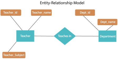
Fig 21: E - R diagram

The above E-R diagram has two entities: Teacher and Department

Teacher entity has three attributes:

Teacher_id

Teacher_name

Teacher_Subject

Department entity has two attributes: -

Dept_id

Dept_name

Relation Teaches in gives relationship between Teacher, Department.

Relationship can be of the type:

1:1 → One to one

1:M   → One to many

M:1   → Many to one

M:M   → Many to many

1.12 Design Issues

We learned how to create an ER diagram in the earlier portions of the data modeling. We also explored various approaches to defining entity sets and their relationships. We also learned how to use different design shapes to represent a relationship, an entity, and its attributes. Users, on the other hand, frequently misunderstand the concept of the elements and the ER diagram's design process. As a result, the ER diagram has a complex structure and some flaws that do not match the characteristics of a real-world business model.

The following are the fundamental design challenges of an ER database schema:

1. Use of Entity Set vs Attributes

The structure of the real-world enterprise being simulated, as well as the semantics associated with its properties, determine the utilization of an entity set or attribute. When a user uses an entity set's primary key as an attribute of another entity set, it results in an error. Instead, he should do so through the relationship. In addition, although the primary key qualities are implied in the relationship set, we designate them in the relationship sets.

2.     Use of Entity Set vs. Relationship Sets

It's tough to tell whether an entity set or a relationship set is the best way to express an item. The user must specify a relationship set for describing an activity that occurs between the entities in order to comprehend and determine the appropriate use. If the object must be represented as a relationship set, it is best to keep it separate from the entity set.

3.     Use of Binary vs n-ary Relationship Sets

The relationships depicted in databases are often binary relationships. Non-binary relationships, on the other hand, can be represented by a number of binary relationships. We can, for example, define and describe a ternary relationship called 'parent,' which can refer to a child, his father, and his mother. Such a relationship can also be represented by two binary partnerships, such as a mother and father who may have a child together. As a result, a set of discrete binary relationships can be used to represent a non-binary relationship.

4.     Placing Relationship Attributes

In the placement of connection qualities, cardinality ratios can become an effective measure. As a result, rather than any relationship set, it is preferable to correlate the attributes of one-to-one or one-to-many relationship sets with any participating entity sets. The choice of whether to place the provided attribute as a relationship or entity attribute should reflect the characteristics of the real-world business being simulated.

For example, rather than determining it as a separate entity, if there is an entity that may be identified by a combination of participating entity sets. Many-to-many relationship sets must be associated with this sort of characteristic.

As a result, it necessitates a thorough understanding of each component involved in designing and modeling an ER diagram. The most basic prerequisite is to examine the real-world enterprise and the relationships between different entities or attributes.

1.13 Extended E-R Features

The Extended Entity-Relationship Model (EERM) is a more abstract and high-level model that expands the E/R model to include more forms of relationships and attributes, as well as to articulate constraints more clearly. The EE/R model includes all of the concepts found in the E/R model, as well as additional concepts that cover more semantic information.

In addition to ER model concepts EE-R includes −

●      Subclasses and Superclasses.

●      Specialization and Generalization.

●      Category or union type.

●      Aggregation.

These concepts are used to create EE-R diagrams.

Key takeaway:

1. EER is a high-level data model that integrates the original ER model's extensions. Enhanced ERD models are high-level representations of the specifications and complexities of complex databases.
2. Generalization/specialization, association, inheritance, and subclass / superclass are some of the additional definitions.

1.14 Converting E-R & EER diagram into tables

Using notations, the database can be represented, and these notations can be reduced to a set of tables.

Each entity set or relationship set can be represented in tabular form in the database.

The ER diagram is given below:

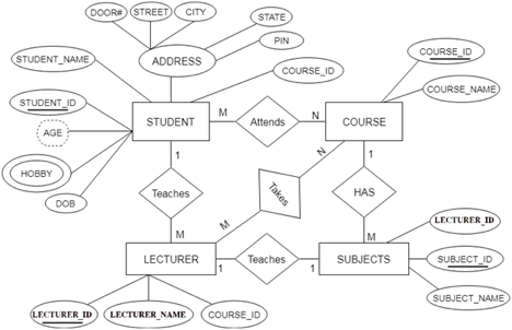
Fig 22: ER diagram

There are some points for converting the ER diagram to the table:

●      Entity type becomes a table.

In the given ER diagram, LECTURE, STUDENT, SUBJECT and COURSE forms individual tables.

●      All single-valued attribute becomes a column for the table.

In the STUDENT entity, STUDENT_NAME and STUDENT_ID form the column of STUDENT table. Similarly, COURSE_NAME and COURSE_ID form the column of COURSE table and so on.

●      A key attribute of the entity type represented by the primary key.

In the given ER diagram, COURSE_ID, STUDENT_ID, SUBJECT_ID, and LECTURE_ID are the key attribute of the entity.

●      The multivalued attribute is represented by a separate table.

A hobby is a multivalued feature inside the student table. Thus, multiple values cannot be expressed in a single column of the STUDENT table. We therefore generate a STUD HOBBY table with the STUDENT ID and HOBBY column names. We create a composite key by using both columns.

●      Composite attribute represented by components.

Student address is a composite attribute in the given ER diagram. CITY, PIN, DOOR#, Path, and STATE are included. These attributes will merge as an individual column in the STUDENT table.

●      Derived attributes are not considered in the table.

In the STUDENT table, the derived attribute is age. It can be determined by measuring the difference between the present date and the date of birth at any time.

You can convert the ER diagram to tables and columns using these rules and assign the mapping between the tables.

The following is the table structure for the given ER diagram:

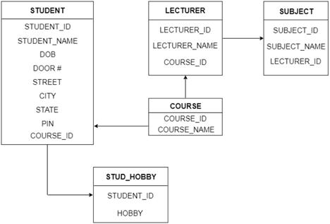
Fig 23: Table structure

Key takeaway:

1. Each entity set or relationship set can be represented in tabular form in the database.
2. Using notations, the database can be represented, and these notations can be reduced to a set of tables.

References:

1. Martin Gruber, “Understanding SQL”, Sybex Publications.
2. Ivan Bayross, “SQL- PL/SQL”, BPB Publications, 4th Edition.
3. S.K. Singh, “Database Systems: Concepts, Design and Application”, Pearson, Education, 2nd Edition.
4. A. Silberschatz, H.F. Korth and S. Sudarshan, “Database System Concepts”, McGraw Hill, 6th Edition.