Unit - 2

Relational Database Design

2.1 Basic concepts

The primary data model is the Relational Data Model, which is commonly used for data storage and processing around the world. This model is simple and has all the features and functionality needed to process data with efficiency in storage.

The relational model can be interpreted as a table with rows and columns. Each row is called a tuple. There's a name or attribute for each table in the column.

Table: Relationships are saved in the format of tables in a relational data model. The relationship between entities is stored in this format. A table includes rows and columns, where rows represent information, and attributes are represented by columns.

Tuple: A tuple is called a single row of a table, which contains a single record for that relationship.

Attributes and Domains

Domain: It includes a set of atomic values that can be adopted by an attribute.

Attribute: In a specific table, it includes the name of a column. Every Ai attribute must have a domain, a domain (Ai)

Relational instance: The relational example is represented in the relational database structure by a finite set of tuples. There are no duplicate tuples for relation instances.

Relational schema: The name of the relationship and the name of all columns or attributes are used in a relational schema.

Relational key: Each row has one or more attributes in the relational key. It can uniquely identify the row in the association.

Example:

STUDENT Relation

●      In the given table, NAME, ROLL_NO, PHONE_NO, ADDRESS, and AGE are the attributes.

●      The instance of schema STUDENT has 5 tuples.

●      t3 = <Laxman, 33289, 8583287182, Gurugram, 20>

2.2 CODD's Rules

After his thorough study into the Relational Model of Database Systems, Dr. Edgar F. Codd came up with twelve rules of his own that, according to him, must be followed by a database in order to be called a true relational database.

These principles can be extended to any database system that only uses its relational features to handle stored data. This is a simple rule that serves as the basis for all the other rules.

1. Information Rule: The data contained in a database must be the value of a table cell, whether it is user data or metadata. It is important to store everything in a database in a table format.
2. Guaranteed Access Rule: Each data element must be accessible by means of the name of the table, its primary key, and the name of the attribute whose meaning is to be determined.
3. Systematic Treatment of NULL values: A systematic and uniform treatment must be given to the NULL values in a database. This is a very relevant rule since it is possible to interpret a NULL as one of the following: information is missing, information is not known or information is not applicable.
4. Active Online Catalog: The definition of the structure of the whole database must be stored in an online catalogue, known as a data dictionary, accessible by registered users. The same query language can be used by users to access the catalogue that they use to access the database itself.
5. Comprehensive Data Sublanguage Rule: A database should be available in a language that is supported for the process of description, manipulation and transaction management.
6. View Updating Rule: Various views that are generated for different purposes should be automatically modified by the framework.
7. High level insert, update and delete rule: High-level addition, upgrading, and removal must be assisted by a database. This must not be limited to a single row, which means that union, intersection and minus operations must also be assisted in order to generate data record sets.
8. Physical data independence: At each relationship level, the Relational Model should support insert, remove, update, etc. operations. Set operations such as Union, Intersection and minus should also be endorsed.
9. Logical data independence: Any alteration of a table's logical or conceptual schema does not involve modification at the level of the application. Merging two tables into one, for example, does not impact access to the application, which is difficult to do.
10. Integrity Independence: Changed integrity restrictions at the database level do not implement changes at the application level.
11. Distribution Independence: For end-users, the distribution of data over different locations should not be noticeable.
12. Non-Subversion Rule: Low level access to data should not be able to circumvent honesty rules to alter data.

Key takeaway:

1. Relational Data Model, which is commonly used for data storage and processing around the world.
2. Each row is called a tuple.
3. There's a name or attribute for each table in the column.
4. These Codd’s rule principles can be extended to any database system that only uses its relational features to handle stored data.

2.3 Relational Integrity: Domain, Referential Integrities, Enterprise Constraints

●      As a description of a valid set of values for an attribute, domain constraints can be specified.

●      The domain data type consists of a string, character, integer, time, date, currency, etc. In the corresponding domain, the value of the attribute must be available.

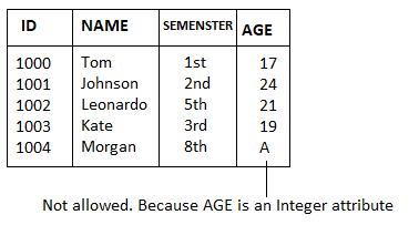
Fig 1: Example of domain constraints

Referential integrity

●      Between two relations or tables, the referential integrity constraints are defined and used to preserve the consistency between the tuples in two relationships.

●      If an attribute of the foreign key of the relationship R1 has the same domain(s) as the primary key of the relationship R2, then the foreign key of R1 is said to refer to or refer to the primary key of the relationship R2.

●      Foreign key values in the R1 relationship tuple can either take the primary key values for a certain R2 relationship tuple, or they can take NULL values, but cannot be zero.

Example

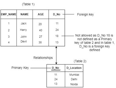
Fig 2: Example of referential integrity

Enterprise constraints

Enterprise constraints are additional rules that users or database managers define and may be based on several tables, often referred to as semantic constraints.

Some explanations are here.

●      There can be a maximum of 30 students for a class.

●      A maximum of four classes per semester can be taught by an instructor.

●      An employee is unable to engage in more than five programmes.

●      An employee's compensation cannot exceed the employee's manager's salary.

2.4 Database Design: Features of Good Relational Designs

In a database, we have numerous relations, as we all know. Each relationship must now be identified separately. If this is not the case, there will be a lot of confusion. We'll go over various features that, if followed, will automatically distinguish a relation in a database.

1. Each database connection must have a different or unique name that distinguishes it from the other database relations.

2. There can't be two attributes with the same name in a relation. Each attribute must be given a unique name.

3. A relation must not contain duplicate tuples.

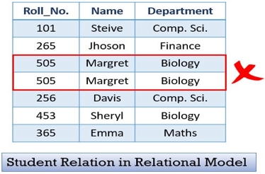
4. For each attribute, each tuple must have precisely one data value. For example, you can see in the first table that we have enrolled two pupils, Jhoson and Charles, for Roll No. 265; this would not work. For each Roll No, we must have only one student.

5. A relation's tuples do not have to be in any particular order because the relation is not order-sensitive.

6. Similarly, the properties of a relation do not have to be in any particular order; the developer can specify how the attributes are ordered.

Key takeaway:

1. Data must be represented as a set of relationships. Each relationship should be clearly depicted in the table.
2. Data about instances of an entity should be contained in rows. Columns must contain information about the entity's attributes.
3. The table's cells should all have the same value. Each column should have its own name.
4. There can't be any two rows that are the same. An attribute's values should all come from the same domain.

2.5 Normalization

Normalization is often executed as a series of different forms. Each normal form has its own properties. As normalization proceeds, the relations become progressively more restricted in format, and also less vulnerable to update anomalies. For the relational data model, it is important to bring the relation only in first normal form (1NF) that is critical in creating relations. All the remaining forms are optional.

A relation R is said to be normalized if it does not create any anomaly for three basic operations: insert, delete and update

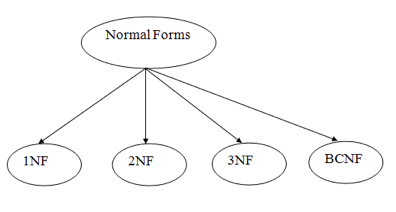
Fig 3: Types of normal forms

1NF

If a relation has an atomic value, it is in 1NF.

2NF

If a relation is in 1NF and all non-key attributes are fully functioning and dependent on the primary key, it is in 2NF.

3NF

If a relation is in 2NF and there is no transition dependency, it is in 3NF.

4NF

If a relation is in Boyce Codd normal form and has no multivalued dependencies, it is in 4NF.

5NF

If a relation is in 4NF and does not contain any join dependencies, it is in 5NF, and joining should be lossless.

Objectives of Normalization

●      It is used to delete redundant information and anomalies in the database from the relational table.

●      Normalization improves by analyzing new data types used in the table to reduce consistency and complexity.

●      Dividing the broad database table into smaller tables and connecting them using a relationship is helpful.

●      This avoids duplicating data into a table or not repeating classes.

●      It decreases the probability of anomalies in a database occurring.

Key takeaway:

1. Normalization is a method of arranging the database data to prevent data duplication, anomaly of addition, anomaly of update & anomaly of deletion.
2. Standard types are used in database tables to remove or decrease redundancies.

2.6 Atomic Domains and First Normal Form

In a relational database, atomic means that it can't be divided any further. Factorization Domain is another name for Atomic Domain. An integral domain is an atomic domain. Atomic domains are distinct from factorization domains with unique factors.

The relational database's Normal Form (NF) gives criteria for identifying the table's degree. 1NF, 2NF, 3NF, and so on are examples of normal forms.

First Normal Form (1NF):

A relation r is in 1NF if and only if every tuple contains only atomic attributes means exactly one value for each attribute. As per the rule of first normal form, an attribute of a table cannot hold multiple values. It should hold only atomic values.

Example: suppose Company has created a employee table to store name, address and mobile number of employees.

In the above table, two employees John, Mary has two mobile numbers. So, the attribute, emp_mobile is Multivalued attribute.

So, this table is not in 1NF as the rule says, “Each attribute of a table must have atomic values”. But in above table the the attribute, emp_mobile, is not atomic attribute as it contains multiple values. So, it violates the rule of 1 NF.

Following solution brings employee table in 1NF.

Key takeaway:

1. A relation r is in 1NF if and only if every tuple contains only atomic attributes means exactly one value for each attribute.

2.6 Decomposition using Functional Dependencies

Functional Dependency (FD) is a constraint in a database management system that specifies the relationship of one attribute to another attribute (DBMS). Functional Dependency helps to maintain the database's data quality. Finding the difference between good and poor database design plays a critical role.

The arrow "→" signifies a functional dependence. X→ Y is defined by the functional dependence of X on Y.

Rules of functional dependencies

The three most important rules for Database Functional Dependence are below:

●      Reflexive law: X holds a value of Y if X is a set of attributes and Y is a subset of X.

●      Augmentation rule: If x -> y holds, and c is set as an attribute, then ac -> bc holds as well. That is to add attributes that do not modify the fundamental dependencies.

●      Transitivity law: If x -> y holds and y -> z holds, this rule is very similar to the transitive rule in algebra, then x -> z also holds. X -> y is referred to as functionally evaluating y.

Types of functional dependency

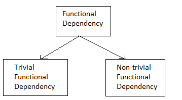
Fig 4: Types of functional dependency

1. Trivial functional dependency

●      A → B has trivial functional dependency if B is a subset of A.

●      The following dependencies are also trivial like: A → A, B → B

Example

Consider a table with two columns Employee_Id and Employee_Name. 

{Employee_id, Employee_Name}   →    Employee_Id is a trivial functional dependency as  

Employee_Id is a subset of {Employee_Id, Employee_Name}. 

Also, Employee_Id → Employee_Id and Employee_Name   →    Employee_Name are trivial dependencies too. 

2. Non - trivial functional dependencies

●      A → B has a non-trivial functional dependency if B is not a subset of A.

●      When A intersection B is NULL, then A → B is called as complete non-trivial.

Example:

ID   →    Name, 

Name   →    DOB 

Key takeaway:

1. The arrow "→" signifies a functional dependence.
2. Functional Dependency helps to maintain the database's data quality.

2.7 Algorithms for Decomposition

By explicitly generating a schema for each dependency in the canonical cover, the decomposition procedure for 3NF ensures that dependencies are preserved. It assures that at least one schema has a candidate key for the one being decomposed, ensuring that the decomposition created is a lossless decomposition.

Decomposition Algorithm

Let Fc be a canonical cover for F;

i=0;

For each functional dependency α->β in Fc

i = i+1;

R = αβ;

If none of the schemas Rj, j=1,2,…I holds a candidate key for R

Then

i = i+1;

Ri= any candidate key for R;

/* Optionally, remove the repetitive relations*/

Repeat

If any schema Rj is contained in another schema Rk

Then

/* Delete Rj */

Rj = Ri;

i = i-1;

Until no more Rjs can be deleted

Return (R1, R2, . . .  ,Ri)

The supplied relation is R, and the given collection of functional dependencies is F, for which Fc maintains the canonical cover. The decomposed portions of the given relation R are R1, R2,..., Ri. As a result, this technique preserves the dependency while also generating a lossless decomposition of R.

A 3NF synthesis algorithm is another name for a 3NF algorithm. It's called so because the regular form works with a dependency set and adds one schema at a time, rather than repeatedly dissecting the basic schema.

BCNF

It is important to check if the given relation is in Boyce-Codd Normal Form before applying the BCNF decomposition technique on it. If it is discovered that the supplied relation is not in BCNF after the test, we can decompose it further to produce BCNF relations.

The following situations necessitate determining whether the supplied relation schema R follows the BCNF rule:

Case 1: Evaluate and compute α+, i.e., the attribute closure of to see if a nontrivial dependency α -> β violates the BCNF rule. Check that + contains all of the attributes of the supplied relation R. It should, therefore, be the super key of relation R.

Case 2: It is not necessary to test all of the dependencies in F+ if the specified relation R is in BCNF. For the BCNF test, all that is required is detecting and checking the dependencies in the specified dependency list F. It's because if no dependent in F violates BCNF, then none of the F+ dependencies will as well.

Decomposition Algorithm

If the supplied relation R is deconstructed into numerous relations R1, R2,..., Rn since it was not found in the BCNF, this algorithm is employed. Thus,

We must validate that α+ (an attribute closure of under F) either includes all the attributes of the relation Ri or no attribute of Ri-α for each subset of attributes in the relation Ri.

Result={R};

Done=false;

Compute F+;

While (not done) do

If (there is a schema Ri in result that is not in BCNF)

Then begin

Let α->β be a nontrivial functional dependency that holds

On Ri such that α->Ri is not in F+, and α ꓵ β= ø;

Result=(result-Ri) U (Ri-β) U (α,β);

End

Else done=true;

This procedure is used to break down a given relation R into its decomposers. This approach does the breakdown of the relation R using dependencies that demonstrate the violation of BCNF. As a result, such an algorithm not only generates relation R decomposers in BCNF, but it is also a lossless decomposition. It signifies that no data is lost when the specified relation R is decomposed into R1, R2, and so on...

The time it takes for the BCNF decomposition procedure to complete is proportional to the size of the original relation schema R. As a result, one disadvantage of this technique is that it may excessively breakdown the given relation R, i.e., over-normalize it.

The decomposition methods for BCNF and 4NF are nearly identical, with one exception. The fourth normal form is concerned with multivalued dependencies, while BCNF is concerned with functional dependencies. The multivalued dependencies aid in reducing data repetition, which is difficult to comprehend in terms of functional relationships.

Key takeaway

1. By explicitly generating a schema for each dependency in the canonical cover, the decomposition procedure for 3NF ensures that dependencies are preserved.
2. It is important to check if the given relation is in Boyce-Codd Normal Form before applying the BCNF decomposition technique on it.
3. If it is discovered that the supplied relation is not in BCNF after the test, we can decompose it further to produce BCNF relations.

2.8 2NF, 3NF, 4NF and BCNF

Second Normal Form (2NF)

A table is said to be in 2NF if both of the following conditions are satisfied:

●      Table is in 1 NF.

●      No non-prime attribute is dependent on the proper subset of any candidate key of table. It means a non-prime attribute should fully functionally depend on the whole candidate key of a table. It should not depend on part of the key.

An attribute that is not part of any candidate key is known as a non-prime attribute.

Example:

Suppose a school wants to store data of teachers and the subjects they teach. Since a teacher can teach more than one subject, the table can have multiple rows for the same teacher.

For above table:

Candidate Keys: {Teacher_Id, Subject}

Non prime attribute: Teacher_Age

The table is in 1 NF because each attribute has atomic values. However, it is not in 2NF because non-prime attribute Teacher_Age is dependent on Teacher_Id alone which is a proper subset of candidate key. This violates the rule for 2NF as the rule says “no non-prime attribute is dependent on the proper subset of any candidate key of the table”.

To bring above table in 2NF we can break it in two tables (Teacher_Detalis and

Teacher_Subject) like this:

Teacher_Details table:

Teacher_Subject table:

Now these two tables are in 2NF.

Third Normal Form (3NF)

A table design is said to be in 3NF if both the following conditions hold:

●      Table must be in 2NF.

●      Transitive functional dependency from the relation must be removed.

So it can be stated that, a table is in 3NF if it is in 2NF and for each functional dependency

P->Q at least one of the following conditions hold:

●      P is a super key of table

●      Q is a prime attribute of table

An attribute that is a part of one of the candidate keys is known as a prime attribute.

Transitive functional dependency:

A functional dependency is said to be transitive if it is indirectly formed by two functional dependencies.

For example:

P->R is a transitive dependency if the following three functional dependencies hold true:

1) P->Q and

2) Q->R

Example: suppose a company wants to store information about employees. Then the table Employee_Details looks like this:

Super keys: {emp_id}, {emp_id, emp_name}, {emp_id, emp_name, Manager_id}

Candidate Key: {emp_id}

Non-prime attributes: All attributes except emp_id are non-prime as they are not subpart part of any candidate keys.

Here, Mgr_Dept, Mgr_Name depend on Manager_id. And, Manager_id is dependent on emp_id that makes non-prime attributes (Mgr_Dept, Mgr_Name) transitively dependent on super key (emp_id). This violates the rule of 3NF.

To bring this table in 3NF we have to break into two tables to remove transitive dependency.

Employee_Details table:

Manager_Details table:

Fourth Normal Form (4NF)

A relation is in the 4NF if it is in BCNF and has no multi valued dependencies.

It means relation R is in 4NF if and only if whenever there exist subsets A and B of the

Attributes of R such that the Multi valued dependency AààB is satisfied then all attributes of R are also functionally dependent on A.

Multi-Valued Dependency

●      The multi-valued dependency X -&gt; Y holds in a relation R if whenever we have two tuples of R that agree (same) in all the attributes of X, then we can swap their Y components and get two new tuples that are also in R.

●      Suppose a student can have more than one subject and more than one activity.

Boyce Codd normal form (BCNF)

It is an advanced version of 3NF. BCNF is stricter than 3NF. A table complies with BCNF if it is in 3NF and for every functional dependency X->Y, X should be the super key of the table.

Example: Suppose there is a company wherein employees work in more than one

Department. They store the data like this:

Functional dependencies in the table above:

Emp_id ->emp_nationality

Emp_dept -> {dept_type, dept_no_of_emp}

Candidate key: {emp_id, emp_dept}

The table is not in BCNF as neither emp_id nor emp_dept alone are keys. To bring this table in BCNF we can break this table in three tables like:

Emp_nationality table:

Emp_dept table:

Emp_dept_mapping table:

Functional dependencies:

Emp_id ->; emp_nationality

Emp_dept -> {dept_type, dept_no_of_emp}

Candidate keys:

For first table: emp_id

For second table: emp_dept

For third table: {emp_id, emp_dept}

This is now in BCNF as in both functional dependencies the left side is a key.

Key takeaway:

1. A relation is in the 4NF if it is in BCNF and has no multivalued dependencies.
2. BCNF is stricter than 3NF. A table complies with BCNF if it is in 3NF and for every functional dependency.

References:

1. A. Silberschatz, H.F. Korth and S. Sudarshan, “Database System Concepts”, McGraw Hill, 6th Edition.
2. Martin Gruber, “Understanding SQL”, Sybex Publications.
3. Ivan Bayross, “SQL- PL/SQL”, BPB Publications, 4th Edition.
4. S.K. Singh, “Database Systems: Concepts, Design and Application”, Pearson, Education, 2nd Edition.