Unit 2
Geometric Modeling
“The curves defined by the analytic equation are defined as analytic curve.”
Examples of analytic curve are:
2.1.1 Lines
Lines are bounded by key-points. They represent edges of object.
A] Lines connecting two end points:
Fig shows a straight line connecting two end points P1 and P2. The parameter ‘u’ is set such that its values are 0 and 1 at points respectively.
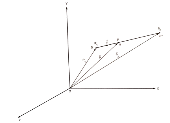
Consider any point P on the line P1P2 with general value of parameter ‘u’.
Let,
 1 be position vector for point P1
 2 be position vector for point P2
 be position vector for point P
From fig


The parametric equation of line is given by

The parametric equation in scalar form is given by


The equation of tangent vector of line P1P2 is

The equation of tangent vector in scalar form is


Unit vector in the direction of line is

Where,

B] Line starting from given point of given length and direction
Let
P1be the starting point of line
 beunit vector in direction of line
L be length of line
The equation of line is given by

Where,

2.1.2 Circles
Fig shows the circle with center (xc, yc, zc) and radius R.
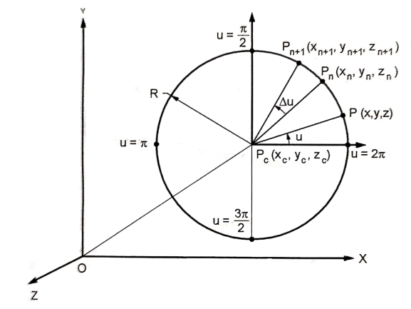
The parametric equation of circle is given as


Where, 
And u = angle measured from X axis to any point P on the circle.
Centre of Circle can be found by


Radius of circle is given by

2.1.3 Circular Arcs
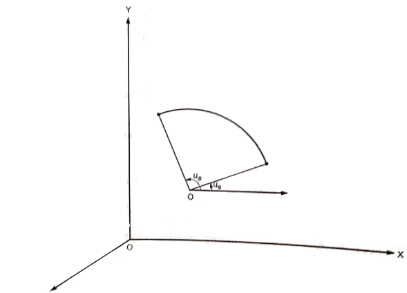
The parametric equation for circular arc with center (xc, yc, zc) and radius R is


Where, 
2.1.4 Ellipses
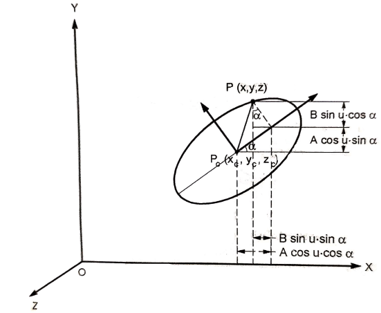
The parametric equation for ellipse is


Where, 
2.1.5 Hyperbola
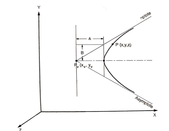
The parametric equation for ellipse is


Where, 
“The curves are defined by the set of data points are called synthetic curves.”
Synthetic curves are in polynomial form
There are two approaches to generate synthetic curve
● Interpolation
In interpolation, the curve passes through all the data points.
● Approximation
In approximation, curve does not pass through all data points but are close to data points.
Major CAD/CAM software uses three types of synthetic curves:
● Hermite Cubic Spline
● Bezier Curve
● B – Spline Curve
2.2.1 Hermite Cubic Spline
A cubic Hermite spline is a spline where each piece is a third-order polynomial specified in Hermite form: that is, by its values and first derivatives at the end points of the corresponding domain interval.
The cubic splines are drawn from two data points and two tangent vectors at these points.
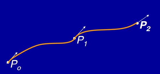
Hermite Spline
A cubic spline are cubic polynomial for their parametric representation and is given by,

General form of parametric equation in any of X, Y or Z directions is

Or 
General parametric equation of Hermite curve passing through two points P0 and P1 and two tangent vectors at these points P0’ and P1’ respectively is

The use of Hermite Cubic Spline in CAD/CAM is not very popular due to its need of two tangent vectors.
2.2.2 Bezier Curves
“The Bezier curves uses the given data points for generating the curve and passes through first and last data points while other acts as control points.”
Bezier curves are used more than Hermite cubic splines because of its flexibility to change shape of curve.
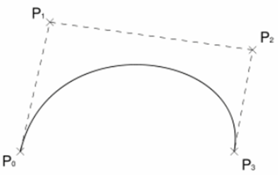
Bezier curve
Parametric equation of Bezier curve is written as,

Or

Where

Bezier curve for n+1 data point is nth degree polynomial.
Characteristics of Bezier curve
● Does not use tangent vectors but data points for controlling its shape
● Bezier curve for n+1 data point is defined by nth degree polynomial.
● The sequence of the data points can be reversed without changing the shape of the curve.
● A closed Bezier curve can be generated by closing its polygon. i.e. End points are made coincident
● The flexibility of Bezier curve increases by increasing data points.
2.2.3 B – Spline Curve
B – Spline Curve separates the degree of polynomial of the curve from the number of data points.
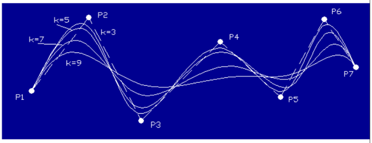
B – Spline Curve
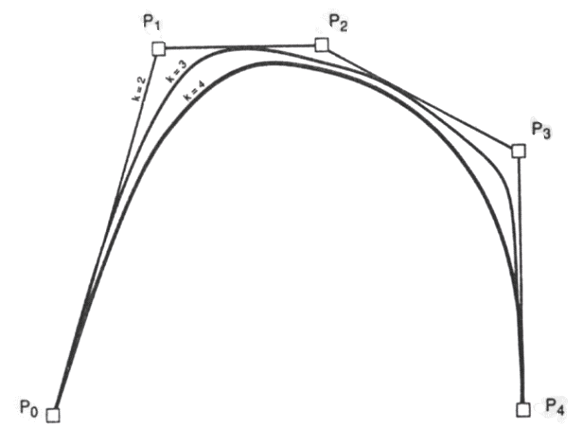
Linear, Quadratic and Cubic B – Spline Curve
“Modeling is the art of representing the object, system or phenomenon.”
There are two types of modeling:
● Geometric modeling
“Geometric modeling is defining as the complete representation of an object with the graphical and non-graphical information.”
● Non-geometric modeling
It is a physical phenomenon
There are three methods of Geometric Modeling
● Wire-Frame Modeling
● Surface Modeling
● Solid Modeling
2.3.1 Wire-Frame Modeling
Wireframe model consists of vertex, edge (line) and polygons. Edge is used to join vertex. Polygon is a combination of edges and vertices. The edges can be straight or curved. This model is used to define computer models of parts, especially for computer-assisted drafting systems.
Wireframe models are Skelton of lines. Each line has two endpoints. The visibility or appearance or look of the surface can be should using wireframe. If any hidden section exists that will be removed or represented using dashed lines. For determining hidden surface, hidden lines methods or visible line methods are used.
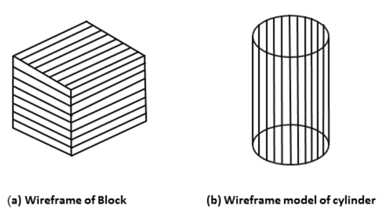
Wire-Frame Modeling
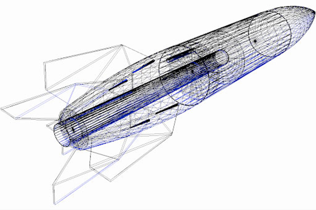
Application of wire-frame modeling
Advantage
Disadvantage
2.3.2 Surface Modeling
Surface Modeling is the method of showing or presenting solid objects. The process requires you to convert between different 3D modeling types, such as converting the 3D object to show procedural surfaces, validate imperfections, and apply smoothness.
While more complex than Wireframe Modeling, Surface Modeling is easier to achieve than Solid Modeling.
In a CAD environment it is possible to fully produce a model using only surface modeling - but most real-world applications require a combination with solid modeling technique as well.
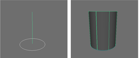
Surface Modeling: Extrusion
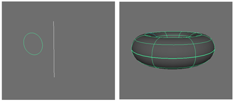
Surface Modeling: Revolution
2.3.3 Solid Modeling
Solid modeling is a set of principles that apply in a computer-aided design (CAD) context, particularly when it comes to simulating 3D objects.
A solid modeling system tries to forecast how the eventual object would look like and ensures that the design of the object is geometrically correct.
Solid modeling has allowed difficult engineering processes to be automated and supports key processes in manufacturing such as machining and assembly.
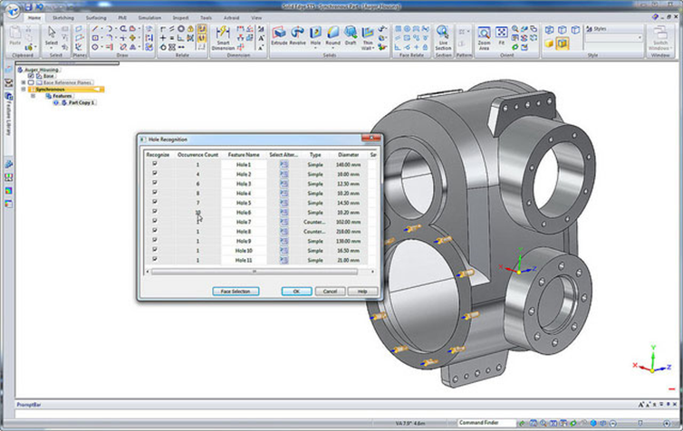
Solid Modeling
The surfaces can be represented by two methods
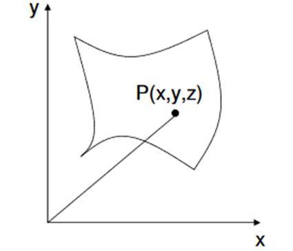
A] Non-Parametric Representation
In general, a surface or surface patch is represented analytically by an equation of the form

Where P is the position vector
The natural choice for f(x,y) is a polynomial.
Thus, for analytical representation of surfaces we can use equations of type

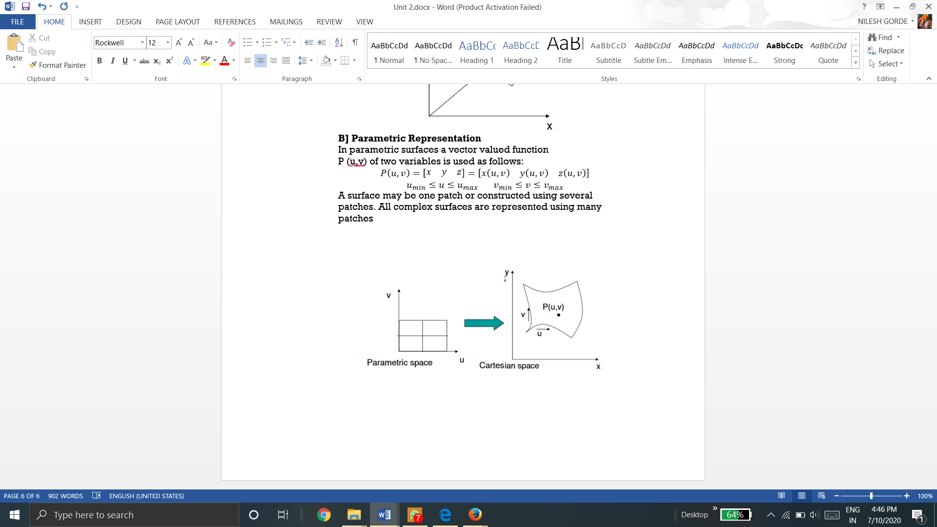
B] Parametric Representation
In parametric surfaces a vector valued function
P(u,v) of two variables is used as follows:


A surface may be one patch or constructed using several patches. All complex surfaces are represented using many patches
Surface entities which are defined by the analytic equation are knows as analytic surface.
The various type of analytic surfaces, used in surface modeling are discussed below:
1) Plane surface
2) Ruled surfaces
3) Tabulated surface
4) Surface of revolution
2.5.1 Plane Surface
This is the simplest surface, requires 3 non-coincidental points to define an infinite plane. The plane surface can be used to generate cross sectional views by intersecting a surface or solid model with it.
Plane Surface
2.5.2 Ruled (lofted) Surface
This is a linear surface. It interpolates linearly between two boundary curves that define the surface. Boundary curves can be any wire frame entity. The surface is ideal to represent surfaces that do not have any twists or kinks.
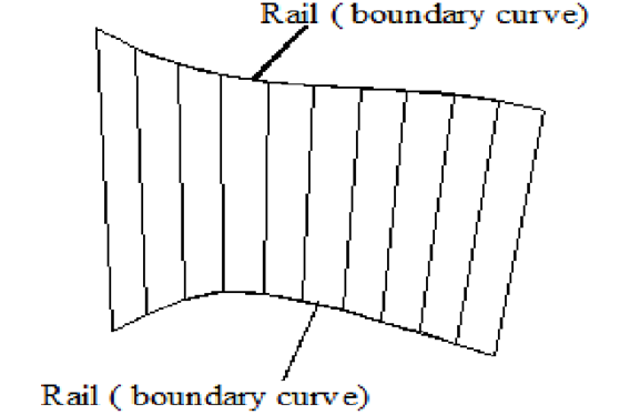
Ruled Surface
2.5.3 Tabulated Surface
This is a surface generated by translating a planar curve a given distance along a specified direction. The plane of the curve is perpendicular to the axis of the generated cylinder.
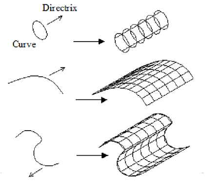
Tabulated Surface
2.5.4 Surface of Revolution
This is an axisymmetric surface that can model axisymmetric objects. It is generated by rotating a planar wire frame entity in space about the axis of symmetry of a given angle.
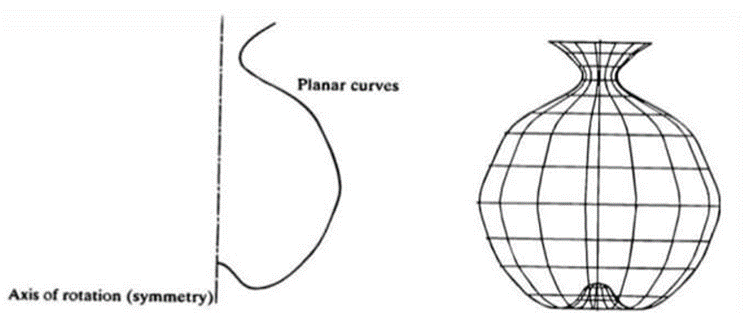
Surface of Revolution
“The surface entities are defined by the set of data point are known as synthetic surfaces.”
The synthetic surfaces are needed when a surface is represented by a collection of data points. The synthetic surface are represented by the polynomial.
The various types of synthetic surfaces, used in surface modeling are:
1) Hermite bi-cubic surface
2) Bezier surface
3) B-spline surface
4) Coons surface(patch)
5) Fillet surface
6) Offset surface
2.6.1 Hermite Bi-Cubic surface
This 3-D surface is generated by interpolation of 4 endpoints. Bi-linear surfaces are very useful in finite element analysis. A mechanical structure is discretized into elements, which are generated by interpolating 4 node points to form a 2-D solid element.
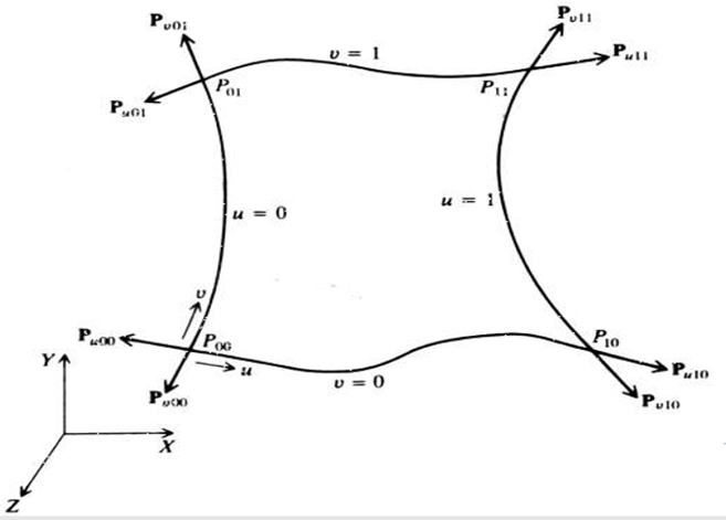
Hermite Bi-cubic Surface
2.6.2 Bezier surface
This is a synthetic surface similar to the Bezier curve and is obtained by transformation of a Bezier curve. It permits twists and kinks in the surface. The surface does not pass through all the data points. It is synthetic surface which is approximated by the given data point.
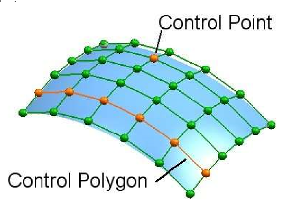
Bezier Surface
2.6.3 B-Spline surface
This is a synthetic surface and does not pass through all data points. The surface is capable of giving very smooth contours, and can be reshaped with local controls.
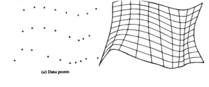
B – Spline Curve
2.6.4 Coons surface(patch)
Coons patch or surface is generated by the interpolation of 4 edge curves as shown
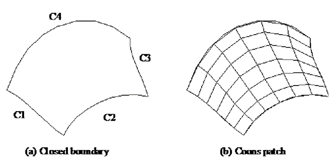
Coons Surface
2.6.5 Fillet surface
Fillet surface is a blend of two surfaces which intersect each other. If required, a fillet of specified radius may be provided at the intersection of two surfaces.
2.6.6 Offset surface
An existing surface can be offset to create new surface. The offset surface is identical in shape with the existing surface, but may have the different dimensions.
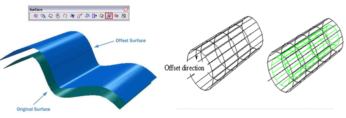
Offset Surface
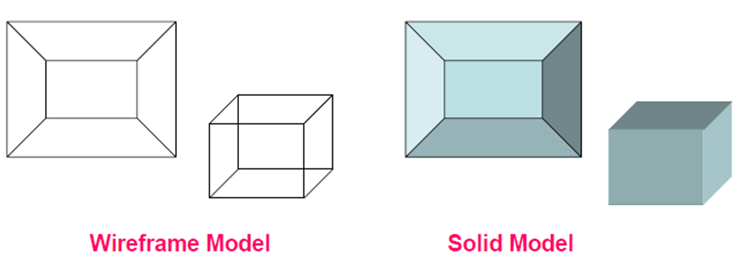
A solid model of an object is a more complete representation than its surface or wireframe model.
It provides more topological information in additional to geometric information which helps to represent the solid unambiguously.
2.7.1 Geometry and Topology
Geometry
Geometry gives a metrics and dimensions of a solid object. It also gives location of object in a chosen coordinate system
Topology
Topology gives a combinatorial information like connectivity, associativity and neighborhood information. It also shows invisible relationship information.
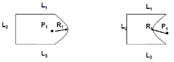
Same Geometry but different topology
2.7.2 Primitive Solid Representation (Solid Instancing)
This is where the objects are defined as a single primitive object and scaled, translated and rotated into the world.
In primitive instancing, all the objects that have same topology but different geometry are grouped into a family called generic primitive. By inputting the values of parameters defining the primitive, the model can be generated.
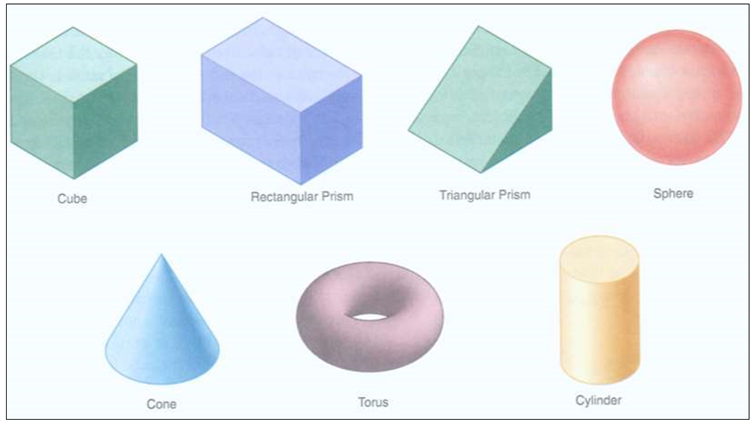
Primitives
Boolean Operations on Primitive
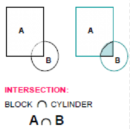
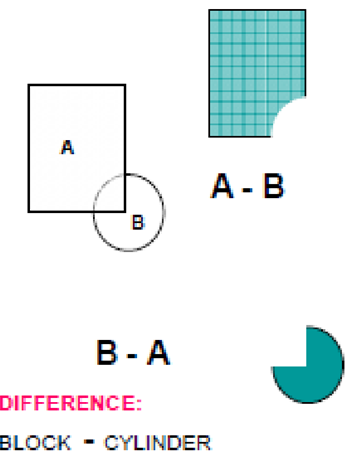
A desired solid can be obtained by combining two or more solids.
When we use Boolean set of operations on two or more primitives, it results into a desired solid geometry.
Normal Boolean operations are union, intersection and subtraction which are given below
1) Union
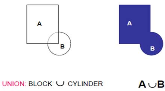
2) Intersection
3) Difference
Application of Boolean equation to create a solid is given below:
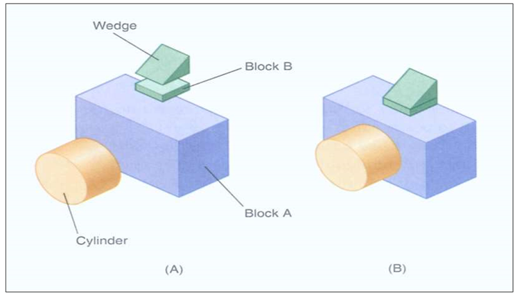
Primitives in use
2.7.3 Boundary representation (B-Rep)
Solid model is defined by their enclosing surfaces or boundaries. This technique consists of the geometric information about the faces, edges and vertices of an object with the topological data on how these are connected.
A solid is represented as a closed space in 3D space (surface connect without gaps). The boundary of a solid separate’s points inside from points outside solid.
B- Rep model
Technique guarantees that surfaces definitively divide model space into solid and void, even after model modification commands.
B-Rep graph store face, edge and vertices as nodes, with pointers, or branches between the nodes to indicate connectivity.
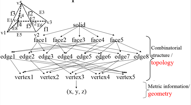
B-rep data structure
B-Rep has to fulfill certain conditions to disallow self-intersecting and open objects.
This condition includes –
● Each edge should adjoin exactly two faces and have a vertex at each end.
● Vertices are geometrically described by point coordinates
● At least three edges must meet at each vertex.
● Faces are described by surface equations
● The set of faces forms a complete skin of the solid with no missing parts.
● Each face is bordered by an ordered set of edges forming a closed loop.
● Faces must only intersect at common edges or vertices.
● The boundaries of faces do not intersect themselves.
Validity of boundary representation by Euler’s Equation:
Validity also checked through mathematical evaluation.
Evaluation is based upon Euler’s Law (valid for simple polyhedral – no hole)
V – E + F = 2 V-vertices E- edges F- face loops
Example:
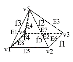
Here, V = 5, E = 8, F = 5
5 – 8 + 5 = 2
Expanded Euler’s law for complex polyhedrons (with holes) • Euler-Poincare Law:
V-E+F-H=2(B-P)
H – number of holes in face,
P- number of passages or through holes,
B- number of separate bodies
2.7.4 Constructive Solid Geometry (C-Rep or CSG)
CSG Tree
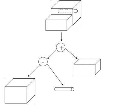
CSG Tree
2.7.5 Boolean Operations on CSG
Boolean operation
– Are intuitive to user
– Are easy to use and understand
– Provide for the rapid manipulation of large amounts of data.
Because of this, many non-CSG systems also use Boolean operations.

2. Intersection

3. Difference

References :
1. Ibraim Zeid, Mastering CAD/CAM – Tata McGraw Hill Publishing Co. 2000
2. Segerling L. J. - Applied Finite Elements Analysis, John Wiley and Sons
3. Seshu P. Text book of Finite Element Analysis, PHI Learning Private Ltd. New Delhi, 2010
4. Rao P. N., Introduction to CAD/CAM Tata McGraw Hill Publishing Co.
5. B. S. Pabla, M. Adithan, CNC Machines, New Age International, 1994
6. Groover M.P.-Automation, production systems and computer integrated manufacturing‘ - Prentice Hall of India
7. Ian Gibson, David W. Rosen, Brent Stucker, Additive Manufacturing Technologies: Rapid Prototyping to Direct Digital Manufacturing, Springer
8. Geoffrey Boothroyd, Peter Dewhurst, Winston A. Knight, Product Design for Manufacture and Assembly, Third Edition ,CRC Press
9. Antti Saaksvuori, Anselmi Immonen, Product Life Cycle Management -Springer, 1st Edition, 2003