UNIT 2

 STATISTICAL CONSIDERATION IN DESIGN

2.1           Introduction to statistical considerations

Statistics is useful in making certain valid conclusions from a set of data out of an experiment or analysis of physical sets. A Few techniques are used for getting data, processing data, analysing data and interpreting it. Decisions are taken based on statistical analysis.

Practically it is difficult to exactly produce components having identical geometric configuration and having functional properties. There are certain variations which occur due to

2.2           Statistical analysis – Terms used

Population is defined as a collection of all elements we are studying and about which we are trying to draw conclusions.

   Eg: Diameters of 10 pins

A sample is defined as a collection of some, but not all, of the elements of the population.

   Eg:

Random variables are of two types:

         Discrete (having unique value)

         Continuous (having variation)

2.3           Frequency Distribution

It is defined as a systematic and organised display of data that shows the number of observation falling into various classes                 

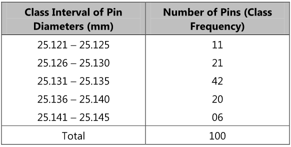
Eg: 25.126 – 25.130

Eg: 21 for interval (25.126 – 25.130)

Eg: 25.130-25.126 = 0.004 mm

Representation of Frequency Distribution

Frequency distribution can be represented by 2 methods

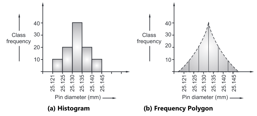
      Histogram is a set of rectangles, base of which is in proportion to the class width and the height in proportion to the class frequency

      Frequency polygon is a graph consisting of lines of class frequency plotted against class marks (mid-point) of class intervals.

2.4           Characteristics of frequency curves

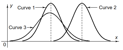
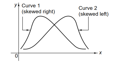
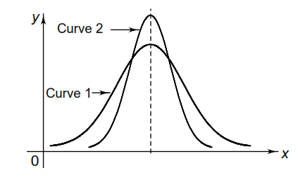
      Central tendency - There is always a central tendency, where most of the observations cluster. “Central tendency is the middle point of distribution”. It is sometimes, referred as the ‘measure of location’. The central location of curve-2 lies to the right of those of curve-1 and curve-3. It is also observed that the central location of curve-1 is equal to that of curve-3.

2.5           Measure of Central Tendency

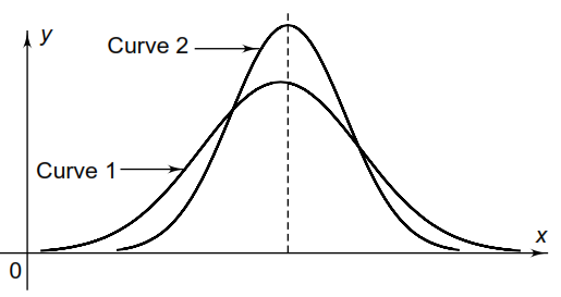
There are different measures of central tendency, such as the mean, the median or the mode. The most popular unit to measure the central tendency is the arithmetic mean denoted by the letter µ. Suppose the population consists of N observations X1, X2,…, XN.

The mean is given by

If observations X1, X2, …, Xk occur f1, f2, …, fk times respectively (i.e., occur with frequencies f1, f2, …, fk), the arithmetic mean is given by

Since, Sfi = N = total number of observations, the mean is given by

The median is the middle item/value, used for qualitative phenomena, and it is given by

item

L – Lower limit, Cf – Cumulative frequency, f –class frequency, i – Class width

The mode is the value of the variety which occurs most frequently in a set of observations, and it is given by

z – Mode

l – Lower limit

h – Width

f1 – Frequency of class

f0 – Frequency preceding

f2 – Frequency succeeding

2.6           Measure of Dispersion(variation of spread)

The dispersion is measured in number of units like the range, the mean deviation or the standard deviation.

Range is the difference between higher and lower value

   Range = (ln –lw)

Mean deviation

The most popular unit for dispersion is the the standard deviation denoted by letter .  The standard deviation is defined as the root mean square deviation from the mean.

When observations X1, X2, …, Xk occur at frequencies f1, f2, …, fk the standard deviation is given by

 Squaring both sides

Using   

  From above equation,

A better estimate of can be obtained by replacing N by (N- 1) in the denominator of the above equation

For values of N > 30, there is little difference between for denominator (N-1) instead of N

 whereis standard deviation

2.7           Standard Normal Curve

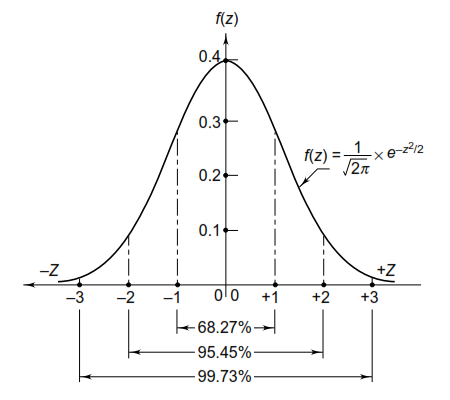
In statistical analysis, the most popular probability distribution curve is the normal curve. The distribution is called normal or Gaussian. The equation of the normal curve in terms of the standard variable Z is given by

An important characteristic of the normal curve is  that  the  total  area  below  the  curve  from  Z = -∞   to   Z = +∞ is one or unity. The areas  included between different values of Z are as follows:

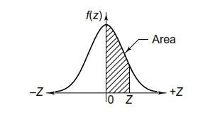
In many design problems, it is required to find out the area below the normal curve from Z = 0 to  a particular value of Z as shown by the shaded area in the figure. The values of this area are given in Table.

Areas under normal curve from 0 to Z

2.8           Population Combinations :

In engineering design problems consisting of two or more populations, it is required to combine these population in certain manner to get a total or effective population.

Eg. Consider population

    A – A population of inner diameter of bearing

    B – The population of outer diameter of shaft

    C – Subtraction of A & B(clearance population)

 Both A & B are random variables.

Condition :

Consider two population as state above, R is the resultant of these two

   µA – Mean of population ‘A’

   µB – Mean of population ‘B’

   µR – Resultant population

   - Standard Deviation of the population ‘A’

   - Standard Deviation of the population ‘B’

   - Standar deviation of the resultant population ‘R’

   CA- Coefficient of variation ‘A’

   CB- Coefficient of variation ‘B’

      Addition of A and B

Mean :       µR = µA + µB

Standard deviation :  

      Subtraction of A and B

Mean :       µR = µA - µB

Standard deviation :  

      Multiplication of A and B :

µR = µA . µB

      Division of A and B :

µR = µA/µB

2.9           Design and Natural Tolerances

The variations in the dimensions of a component occur due to two reasons—first, because of a large number of chances causes and, second, due    to assignable causes. The variations due to chance causes occur at random. They are the characteristics of the manufacturing method and measurement technique. The variations due to assignable causes can be located and corrected. When they are corrected, the system is said to be under ‘statistical control’.

In a statistically controlled system, the dimensions of the component are normally distributed with a particular value of standard deviation. The natural  tolerance  is  defined  as the actual capabilities of the process, and can be considered as limits within which all but a given allowable fraction of items will fall.  In general, the natural tolerance of a process is the spread of the normal curve that includes 99.73% of the total population. Referring  to  the  normal  curve,  the values of the standard variables Z1 and Z2 corresponding to this population are –3 and +3.

   X = m + Z

Therefore,  X1 = m + 3() and X 2  = m - 3()

Therefore, the natural tolerances are 3 ( ).

On the contrary, the design tolerances are specification limits, set somewhat arbitrarily  by  the designer from considerations of the proper matching of the two components and functioning  of the assembly. The design tolerances can be achieved only when the manufacturing process is so selected that the natural tolerances are within  the design tolerances. The percentage of rejected components depends upon the relationship between these two tolerances. Based on this relationship, the following observations are made:

        When  the  design  tolerance  is  less  than  ( 3 ), the percentage of rejected components is inevitable.

        When the design tolerance is equal to (3 ), there is virtually no rejection provided that the manufacturing process is centered.  For an off-center process, some components are rejected.

        When the design tolerance is slightly greater than (3 ), there is no rejection even if the manufacturing process is slightly off-center.

It is necessary for the designer to select a manufacturing process for a component in such a way that the natural tolerance of the process is slightly less than design tolerance. The design tolerance should be about ( 4 ).

2.10     Machine reliability and Factor of Safety

      Elements of Reliability :

      Relation between Reliability and quality :

      Factor of safety

A factor of safety mainly focus on the following points in the design of a products:

Therefore FOS does not address reliability; sometimes probabilistic approach is used to design a component for a given magnitude of reliability.

Reference books: