Unit 2
Curves & Surfaces
Geometric entities like point, line and circle can be defined by various methods. Some of these methods are shown below.
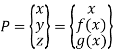
In cartesian Method a point in 2D system is defined by coordinates of that point like

Where x is the distance of point from y axis or projection of point on x-axis while y is the distance of point from x-axis or projection of point on y-axis.
In 3D system, point is defined by

Line is defined by a quadratic equation such as
In the above equation, for every value of x the corresponding value of y coordinate can be found out to get the point.
A circle is defined by a 2nd order function
Where, (a, b) represents the center of the circle and r is the radius of circle.
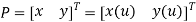
2. Matrix Method
Matrix method is another method of representing the geometric entities.
Point in matrix method is defined like

Or

Circle or line in matrix method, are again defined by the points on the circle or line. The points are given by


These are the two most widely used methods in geometric modelling.
More methods for defining geometric entities are vector, scalar, etc.
Curves can be described mathematically by nonparametric (cartesian) or parametric equations. Nonparametric equations can be explicit or implicit.
i.e curve can be mathematically represented as
For a nonparametric curve, the coordinates y and z of a point on the curve are expressed as two separate functions of the third coordinate x as the independent variable.
In other words, in non-parametric or cartesian system, the curve is represented as a relation between the coordinates x, y, z.
There are two forms of non-parametric representation of curves:
In explicit representation, coordinates are expressed as a function of any one independent coordinate.
Explicit Non-parametric representation for 2D curve is
Explicit Non-parametric representation for 3D curve is

b. Implicit representation
In implicit representation, the curve is represented as a relation between the coordinates.
Implicit Non-parametric representation for 2D curve is

Implicit Non-parametric representation for 2D curve is


Limitation of non-parametric or cartesian or generic representation of curves:
2. Parametric Representation
All the difficulties in non-parametric representation are overcome in parametric representation.
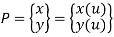
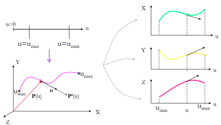
In parametric form, each point on a curve is expressed as a function of a parameter u.
Here, the coordinates are not in relation with each other but are the function of an independent parameter u [f(u)].
This independent coordinate acts as a local coordinate for the points on the curve.
Parametric representation for 2D curve is


Where, 
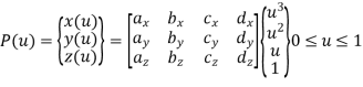
Parametric representation for 2D curve in matrix form is
Where, 
The tangent vector at point P is


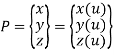
Parametric representation for 3D curve is


Where, 
Parametric representation for 2D curve in matrix form is

Where, 
The tangent vector at point P is


The basic geometric curves used in wire-frame modelling are divided into two types:
“The curves defined by the analytic equation are defined as analytic curve.”
Analytic curves are used for representing profiles of various engineering entities and components.
Examples of analytic curve are:
2. Synthetic Curves
“The curves are defined by the set of data points are called synthetic curves.”
Synthetic curves are in polynomial form.
The synthetic curves are used for representing profiles of car, bodies, ship hulls, etc.
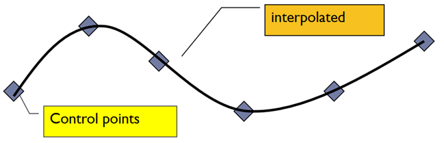
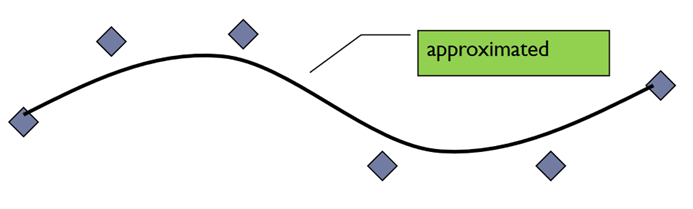
There are two approaches to generate synthetic curve
In interpolation, the curve passes through all the data points.
In approximation, curve does not pass through all data points but are close to data points.
Examples of synthetic curves are
Lines are bounded by key-points. They represent edges of object.
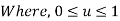
A] Lines connecting two end points:
Fig shows a straight line connecting two end points P1 and P2. The parameter ‘u’ is set such that its values are 0 and 1 at points respectively.
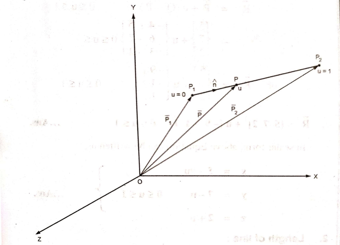
Consider any point P on the line P1P2 with general value of parameter ‘u’.
Let,
 1 be position vector for point P1
 2 be position vector for point P2
 be position vector for point P
From fig

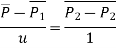
Therefore, the parametric equation of line is given by
The parametric equation in scalar form is given by
The equation of tangent vector of line P1P2 is

The equation of tangent vector in scalar form is


Unit vector in the direction of line is
Where,

B] Line starting from given point of given length and direction
Let
P1 be the starting point of line
 be unit vector in direction of line
L be length of line

The equation of line is given by

Where,

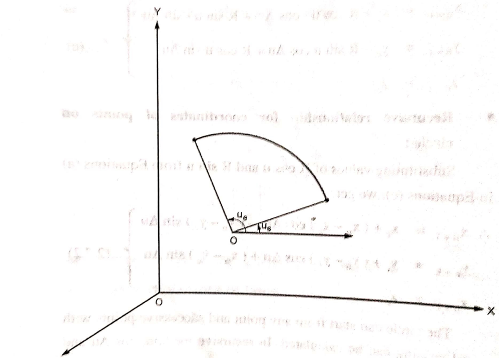
2. Circle
Circles and circular arcs are among the most common entities used in wireframe modeling
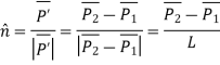
Fig shows the circle with center (xc, yc, zc) and radius R.
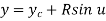
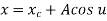
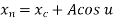
The parametric equation of circle is given as


Where, 
And u = angle measured from X axis to any point P on the circle.
The parametric equation of circle in incremental or recursive form is:

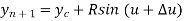

Where, 
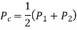
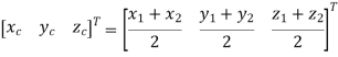
Centre of Circle can be found by
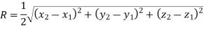
Radius of circle is given by
Circular Arc:
Fig shows the circle with center (xc, yc, zc) and radius R
The parametric equation for circular arc with center (xc, yc, zc) and radius R is


Where, 
3. Ellipse
Figure below shows an ellipse with point Pc (xc, yc, zc) as the center while A and B as semi-major and semi-minor axis respectively.
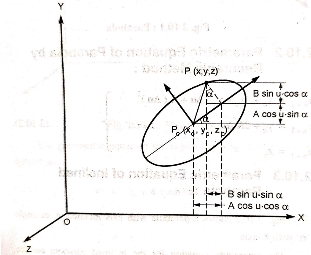
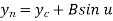
The parametric equation for ellipse is
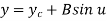

Where, 
The parametric equation of ellipse in incremental or recursive form is

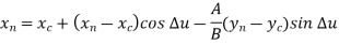
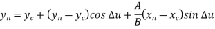

Where, 
Most often, a complex is modeled by several curve segments pieced together end to end.
This is the approach of “segmentation” because each time we analyzing a “curve segment” rather than the entire curve
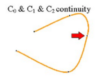
Continuity at the joints of curve segments decides the degree smoothness of the curve
Various continuity requirements –Co, C1, C2 –can be specified as indication of degree smoothness.
To ensure a smooth transition from one section of a piecewise parametric curve to the next, we can impose various continuity conditions at the connection points.
A C1 curve is the minimum acceptable curve for engineering design. A cubic polynomial is the minimum-order polynomial that can guarantee the generation of C0, C1 or C2 curves
If each section of a spline is described with a set of parametric coordinate functions of the form


Where, 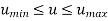
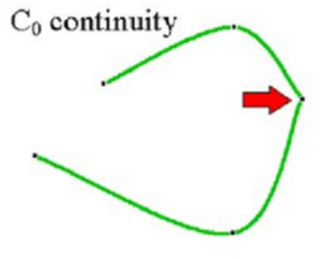
Zero-order parametric continuity, described as C0 continuity, means simply that the curves meet.
The end points of the two curve segments meet with each other in C0 continuity.
Zero-order continuity C0 yields a position continuous curve.
That is, the values of x, y, and z evaluated at u, for the first curve section are equal, respectively, to the values of x, y, and z evaluated at u, for the next curve section.
Mathematically,
(x, y, z for curve segment 1 at u = umax) = (x, y, z for curve segment 2 at u = umin)
2. First order continuity C1
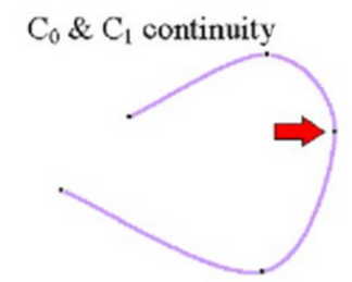
First-order parametric continuity, C1 continuity, means that the first parametric derivatives (tangent lines) of the coordinate functions for two successive curve sections are equal at their joining point.
C1 continuity imply slope continuous curves
At the joining of two segments, the tangent or first order derivative of parametric equation of both curve segment coincides or are equal.
Mathematically,
(x’, y’, z’ for curve segment 1 at u = umax) = (x’, y’, z’ for curve segment 2 at u = umin)
3. Second Order Continuity C2
Second-order parametric continuity, or C2 continuity, means that both the first and second parametric derivatives of the two curve sections are the same at the intersection.
C2-order continuity imply curvature continuous curves.
At the joining of two segments, first order derivative as well as second order derivative of parametric equation of both curve segment coincides or are equal.
Mathematically,
(x’’, y’’, z’’ for curve segment 1 at u = umax) = (x’’, y’’, z’’ for curve segment 2 at u = umin)
Need of Synthetic curve
There are two approaches to generate synthetic curve
In interpolation, the curve passes through all the data points.
In approximation, curve does not pass through all data points but are close to data points.
Some of the synthetic curves used in CAD are:
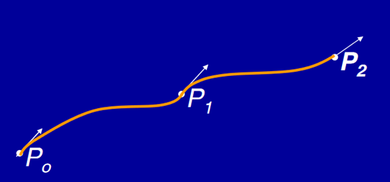
A cubic Hermite spline is a spline where each piece is a third-order polynomial specified in Hermite form: that is, by its values and first derivatives at the end points of the corresponding domain interval.
The cubic splines are drawn from two data points and two tangent vectors at these points.
Hermite Spline
A cubic splines are cubic polynomial for their parametric representation and is given by,
General form of parametric equation in any of X, Y or Z directions is

Or 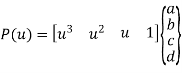
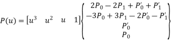
General parametric equation of hermite curve passing through two points P0 and P1 and two tangent vectors at these points P0’ and P1’ respectively is
The use of Hermite Cubic Spline in CAD/CAM is not very popular because it need two tangent vectors.
2. Bezier Curve
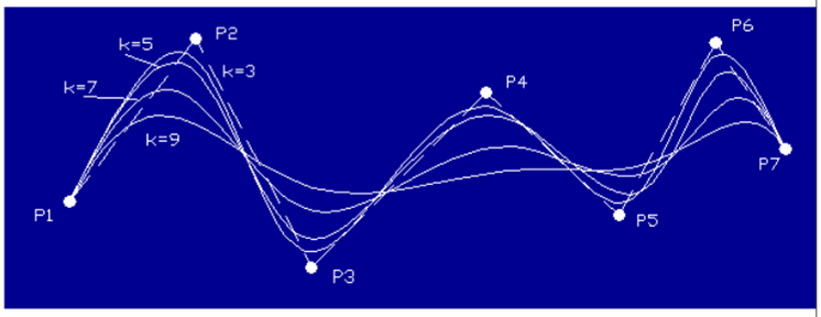
“The Bezier curves uses the given data points for creating the curve and which passes through first and last data points and points other acts as control points.”
Bezier curves are used more than hermite cubic splines because of its flexibility to change shape of curve.
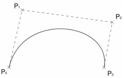
Bezier curve
Parametric equation of Bezier curve is written as,
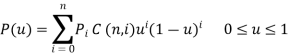
Or
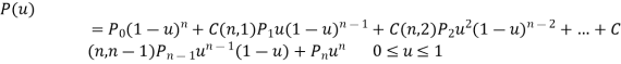
Where
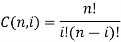
Bezier curve for n+1 data point is nth degree polynomial.
Characteristics of Bezier curve
3. B-spline Curve
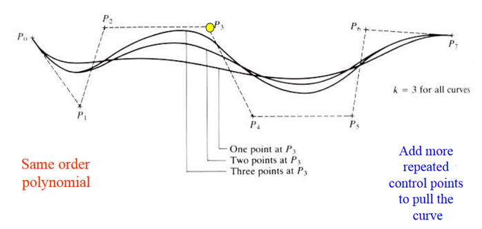
B – Spline Curve separates the degree of polynomial of the curve from the number of data points.
B – Spline Curve
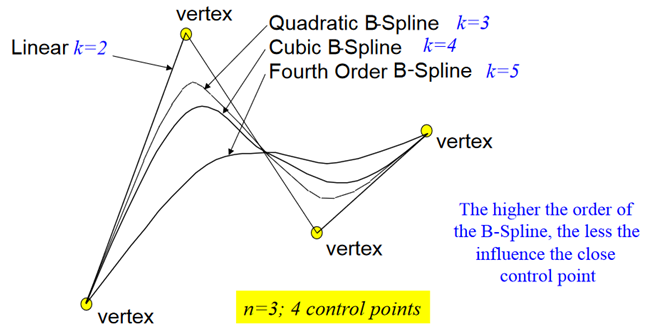
Linear, Quadratic and Cubic B – Spline Curve
A B-spline curve P(t), can be defined by
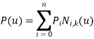
where
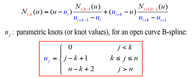
where, 
Thus if a curve with (k-1) degree and (n+1) control points is to be developed, (n+k+1) knots then are needed with 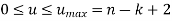
The order k does not depend of the number of control points (n + 1). In the B-Spline curve one have the flexibility of using many control points, and restricting the degree of the polynomial segments.
4. Non Uniform Rational B-spline (NURBS) curve
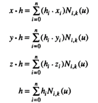
A nonuniform rational B-spline curve, or simply a NURBS curve, is similar to a nonuniform B-spline curve in that it uses the same blending functions derived from the nonuniform knots as those of nonuniform B-spline curves. However, the control points are given in the form (xi h i, y i h i, z i h i, h i), using the homogeneous coordinates h; instead of (x i, y i, z i), and these four coordinates are blended by the blending functions. Thus the coordinates of a point on a NURBS curve in the homogeneous space; (x · h, y · h, z · h, h), are obtained from
The x, y, and z coordinates of a point can be obtained by dividing x · h, y · h, and z · h by h, so the equation of NURBS curve P(u) is derived as
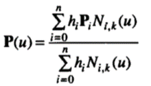
where Pi is a position vector composed of (x i, y i, z i), which are the x, y, and z coordinates of the ith control point in three-dimensional space, as for the nonrational B-spline curves. The parameter interval of the curve is 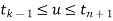 as in the B-spline curve in the preceding section.
Properties of NURBS curve
Representation of surfaces is an extension of the representation of curves.
Similar to curves, the surfaces can be represented by two methods
A] Non-Parametric Representation
A surface or surface patch is represented analytically by an equation of the form

Where P is the position vector
In matrix form the equation is
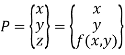
The natural choice for f(x,y) is a polynomial.
Thus for analytical representation of surfaces we can use the following type of equations

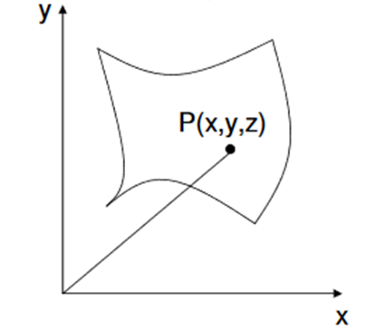
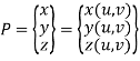
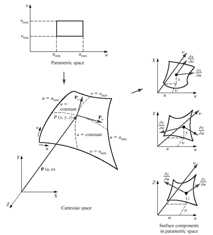
B] Parametric Representation
Just like in case of curves, for surface also parametric representation is widely used. In parametric representation, each point on a surface is expressed not as a relationships between x, y, z but as a function of independent variables u and v.
In parametric surfaces a vector valued function
P (u,v) of two variables is used as follows:


u, v act as a local coordinates for points on the surface or surface Patch.
In matrix form the equation is
A surface can be of one patch or it can be constructed using several patches. All the complex surfaces are represented using many patches
Similar to curves, surfaces are also classified into two categories
Surface entities which are defined by the analytic equation are knows as analytic surface.
The various type of analytic surfaces that are used in surface modeling are given below:
This is the simplest surface that needs 3 non-coincidental points to define an infinite plane. The plane surface can be used to create cross sectional views by intersecting a surface or solid model with it.
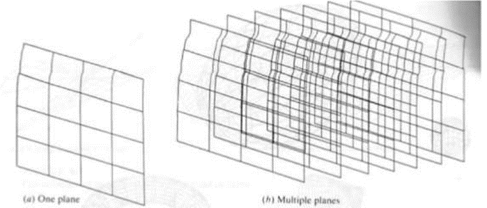
Plane Surface
2. Ruled (lofted) Surface
This is a linear surface which interpolates linearly between two boundary curves that defines the surface. Boundary curves may be any wire frame entity. The surface is ideal to represent surfaces that dont have any twists or kinks.
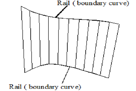
Ruled Surface
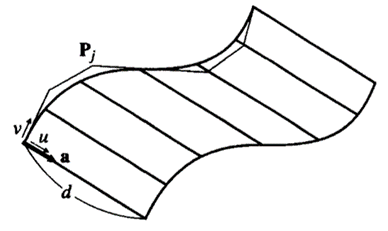
3. Tabulated Surface
This is a surface generated by translating a planar curve with a given distance in a specified direction. The plane of the curve should be perpendicular to the axis of the generated cylinder.
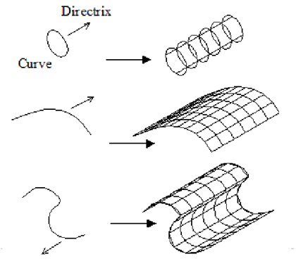
Tabulated Surface
4. Surface of Revolution
This is an axisymmetric surface that is used to model axisymmetric objects. It is generated by rotating a planar wire frame entity about the axis of symmetry of a given angle.
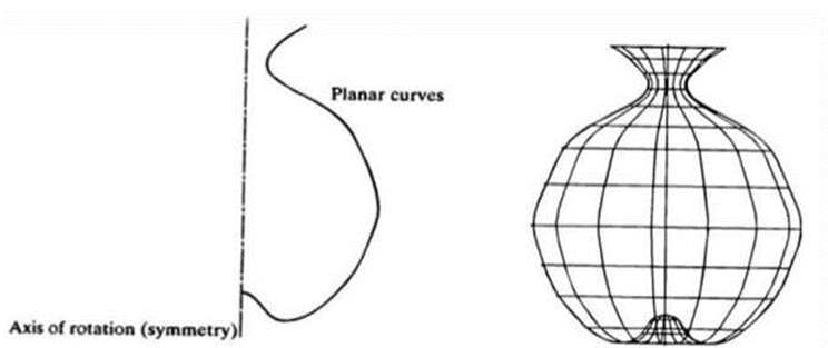
Surface of Revolution
B. Synthetic surfaces
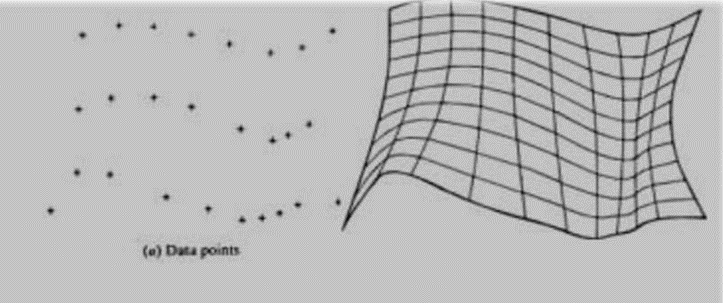
“The surface entities are defined by the set of data point are known as synthetic surfaces.”
The synthetic surfaces are needed when a surface is represented by a collection of data points. The synthetic surface are represented by the polynomial.
The various types of synthetic surfaces, used in surface modeling are:
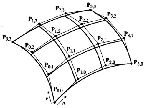
We can extend the concept of defining a curve by a control polygon in a Bezier curve to one dimension higher so that a surface is defined by a control polyhedron. The equation of this surface, called a Bezier surface, is
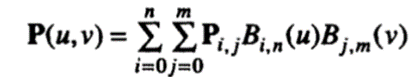
where Pi,j are the control points at the vertices of the control polyhedron, as illustrated in Figure 7.4, and Bi,n and Bj.m are the blending functions used in Bezier curves. Thus, the degree of the surface equations in u and v are determined by the number of control points in the respective directions.
Bezier surface is derived if the control points in a Bezier curve are replaced with Bezier curves.
The degree of a Bezier surface is determined by the number of the control points. As higher degree surface equations have the same problem as higher degree curve equations, we usually use a Bezier surface of degree 3 in both u and v in modeling surfaces, just as we use a Bezier curve of degree 3. Thus, when the surface to be modeled is complicated, it may sometimes be necessary to create several Bezier surfaces of degree 3 and join them. In that case, we want to join the surfaces so that they look continuous across the common boundary. This can be achieved by constraining each pair of the left-hand side and right-hand side control points around the common boundary to form a straight line passing through the control point of the common boundary, as illustrated in Figure.
2. B-Spline Surface
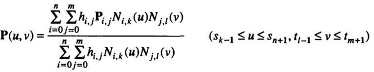
As we have extended the Bezier curve equation to that of a Bezier surface, we can also extend the B-spline curve equation to derive the equation of a B-spline surface:
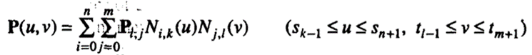
where Pi,j are the control points located at the vertices of the control polyhedron, as for the Bezier surface, and Ni,k(u) and Nj,l(v) are the blending functions used in B-spline curves.
These blending functions are defined by the knot values s0, s1,…, sn+k and t0, t1,…, t1+m, respectively.
The parameter ranges  are used because the blending functions Ni,k(u) and Nj,l(v) are defined only over these intervals.
This is true also when the blending functions are based on periodic knots as well as on nonperiodic knots. Here we consider only the blending functions based on nonperiodic knots, as we did for B-spline curves. In this case, these blending functions become the same as those of Bezier surfaces if the orders k and 1 equal (n + l) and (m+ l), respectively.
When the definition of a B-spline surface is based on nonperiodic knots, it has properties similar to those of a Bezier surface (i.e., the four corner points of the control polyhedron lie on the surface, and the boundary curves are B-spline curves defined by the proper subsets of the control points). Let's now show that the boundary curve corresponding to u = 0 is a B-spline curve. Substituting u = 0 in Equation yields,
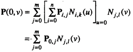
According to Equation (7.33), the boundary curve corresponding to u = 0 is a B-spline curve whose control points are P0,0, P0,1,…, P0,m· Similarly, we can show that the remaining three boundary curves are also B-spline curves and that their control points are the external vertices of the control polyhedron of the surface.
B-spline surface does not pass through all data points. The surface is capable of giving very smooth contours, and can be reshaped with local controls.
B-spline surface
3. NURBS surface
NURBS curve equation can be derived from the B-spline curve equation by introducing homogeneous coordinates for the control points. Similarly, we can derive equation of a NURBS surface from that of a B-spline surface:
where Pi,j are the x, y, and z coordinates and hi,j are the homogeneous coordinates of the control points.
Above equation becomes a B-spline surface when all hi,j equal l, as for the NURBS curve equation.
The NURBS surface equation is a general form that includes the B-spline surface equation. Furthermore, the NURBS surface equation has the advantage of exactly representing the quadric (or quadratic) cylindrical, conical, spherical, paraboloidal, and hyperboloidal surfaces. These surfaces are called quadric (or quadratic) because their surface equations have degree 2 in the parameters u and v. Therefore, the NURBS surface equation often serves as a unified internal representation for all these surfaces.
The NURBS curve of interest has order 1, knot values t (p = 0, l,..., m+ 1), and (m+l) control points specified by Pj, the x, y, and z coordinates, and the homogeneous coordinates hj, as in the following equation. Thus,
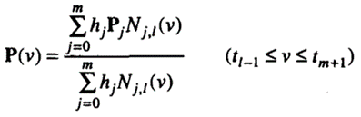
A boundary curve of a NURBS surface is a NURBS curve defined by control points; these control points are the boundary vertices of the control polyhedron associated with the boundary curve. Also, the order and the knots of the boundary curve are the same as for the surface in the corresponding direction.
4. COON'S Patch Surface
The corner points are blended in a bilinear surface, but four boundary curves are blended to form a surface in a Coon's patch. The word patch is used to indicate explicitly that the surface being generated is a surface segment corresponding to the parameter region 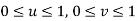 . Thus, any arbitrary surface is composed by many of these patches.
The equation of a Coon's patch is derived as follows. We assume that the equations of the four boundary curves are given by P0(v), P1(v), 'Q0(u), and Q1(u), as illustrated in Figure.
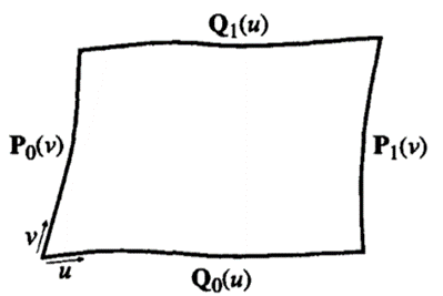
We also assume that the curves 'lo(u) and Q1(u) have the interval of u from 0 to 1 and the same direction. In Figure, we assume that their direction is to the right, as indicated by the arrow for u. Similarly, P0(v) and P1(v) have the interval of v from 0 to 1 and the same direction, upward in this case.
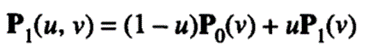
First, two curves facing each other are selected, say, P0(v) and P1 (v). Then they are interpolated in the u direction by a linear equation:
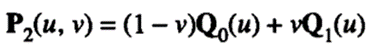
Now let's try to define another surface by interpolating Q0(u) and Q1(u) in the v direction:
Now, let's try yet another surface, P3(u, v), defined by adding P1(u, v) and P2(u, v) to determine whether it can be bounded by all the boundary curves. Then P3(u, v) becomes

and substituting the limit values of u and v
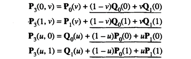
Each underlined term is the linear interpolation between the end points of the corresponding boundary curve. In other words, the terms to be eliminated are the expressions of the boundary curves of a bilinear surface
Therefore, the correct equation of a Coon's patch is obtained by subtracting the bilinear surface equation from P 3(u, v):

The method of representing solid objects is Surface Modeling. The process needs to convert different 3D modeling types, like, validate imperfections, conversion of the 3D object to show procedural surfaces and apply smoothness to the surface. The skin of an object is referred by a surface model. These skins don’t have thickness or material type.
This type of modeling is complex than Wireframe Modeling but Surface Modeling is easier than Solid Modeling.
In a CAD, generation of a full model using only surface modeling is possible - but most real-world applications need a combination of solid modeling and surface modeling.
As it defines the edges of a 3D object and also its surfaces, hence, Surface modeling is easier than wireframe modeling. Surface models defines the surface features and the edges, of objects. A mathematical function describes the path of a curve as in parametric techniques.
A surface model gives an adequate data on a component’s surface geometry. Hence, hidden lines and surfaces are automatically removed as required. This gives rise, when viewed from any direction, to non-ambiguous visualization of the object. The amount of light reflected back to the user from different areas on the surface are calculated by CAD software and each area is color filled with different shades.
Complex objects such as car or airplane body cannot be achieved utilizing wireframe modeling.
Surface modeling is used in
Advantages
Disadvantages
Applications
The process from which a geometric CAD model is obtained from measurements which are acquired by scanning an existing physical model is referred to Reverse engineering. The measurements are in the form of 3D point clouds. These measurements correspond to re-engineered points on the surface of the object. In various industries, CAD models help improve the quality and efficiency of design. Hence, they are very important to represent the scanned object. Also, speed of the manufacturing and analysis process is increased.
Reverse engineering is widely used for various reasons. One can obtain the CAD model of a part which is not manufactured by its manufacturer or the part whose only traditional blueprints exist. This is possible by reverse engineering. Also, there exists the cases where the original CAD model doesn’t refer to the physical part which was manufactured. This was due to subsequent undocumented modifications that were made after the initial design stage. Stylists and artists usually create physical models of their concepts. This is done by using clay, plaster or wood. Then, at an industrial scale, to create CAD models for manufacturing the objects, these models are used.
Jewelry reconstruction is an application of reverse engineering. Jewelry design is a conceptual and decorative type of design.
Reverse Engineering is widely used in numerous applications, such as industrial design and jewelry design, manufacturing, and reproduction. For manufacturing, the use of feature-based constraint-based representations is more appropriate. This is because they capture design intent. Firstly, in order to describe point cloud, some candidate features are extracted. Then, to describe the solid object, these features are reconstructed. Constraints can be detected and maintained automatically, also design intent is captured by providing robustness guaranties. In order to describe repeated patterns common to different types of traditional jewelry, Voxel inspired techniques are also used.
Reverse Engineering Methodology
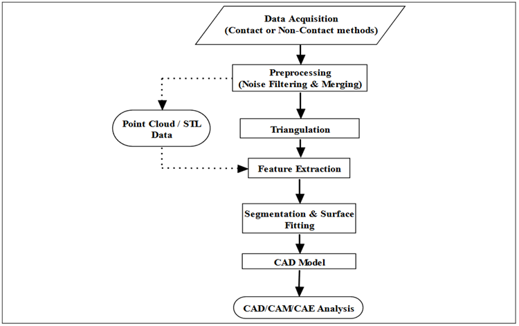
Now-a-days, on different methodologies of reverse engineering attention is focused. The state of the art in reverse engineering is to reconstruct true geometric shape from physical objects in an efficient and accurate way. The typical procedure of reverse engineering shown in the figure below.
Reverse Engineering
It consists of five steps:
(1) data acquisition,
(2) preprocessing (noise filtering and merging),
(3) triangulation,
(4) feature extraction, and
(5) segmentation and surface fitting.
Data acquisition and processing systems includes hardware and software components. point clouds or volumetric data are acquired by a hardware system. This is done with the use of available experimental setup. A software system processes raw point clouds or volumetric data and transfers them into a virtual representation of object surfaces. The point cloud data is acquired in the form of x, y and z co-ordinates of the multiple point of the object surface. The scanning techniques use to scan the object are divided into two types: contact and noncontact technique.
3D digitization system such as non-contact 3D scanner generated the large amount of data. In general, scanning data can be saved in different file formats, out of which the point cloud and STL formats are very useful for research assessment.
Most widely known issues in reverse engineering are STL data and Point cloud. Noise is everywhere in measured data. Therefore, it is important to prepare the noise free scanned data before the surface reconstruction process. This preparation is known as preprocessing.
In digitization system, surface reconstruction methods and pre-processing phase are different processes. For the pre-processing the steps are given below:
Splitting of a triangular mesh into sub-meshes where an appropriate single surface can be fitted is done in the segmentation process. And the quality of the resulting CAD model is affected.
It is essential to make the use of features (sharp edges and symmetry planes) which are extracted in the fourth step to improve the quality of segmentation,. Among various features, few features are very important for the segmentation process because of them, some feature properties are directly applied in industrial products. A concept with redesign and prototyping of free-form surfaces in the manufacturing industry often involves.
Point Cloud Data
A point cloud is nothing but a collection of data points defined by a given coordinates system. Point clouds are used to generate 3D meshes. PCD can also be used to create models that are used in 3D modeling for different fields involving 3D printing, manufacturing, medical imaging, architecture, 3D gaming and different virtual reality (VR) applications. For example in a 3D coordinates system, a point cloud can be used to define the shape of some real physical system
In a 3D cartesian coordinate system, a point is identified by 3 coordinates which relate to a precise point in space relative to a point of origin if taken together. X, y and z axes extended in two directions The coordinates identifies the distance of the point from the intersection of the axes (0) and the direction of divergence. It is generally expressed as ‘+’ or ‘-‘
3D scanners acquire point measurements from real-globe objects or photos for a point cloud which are to be translated to a 3D mesh or NURBS or CAD model.
In simple words, Point clouds are datasets that represent objects or space. These points constitute the X, Y, and Z geometric coordinates of a one point on an underlying sampled surface. The point cloud becomes 4D when colour information is present.
Point clouds are most commonly generated using 3D laser scanners and LiDAR (light detection and ranging) technology and techniques. Here, a single laser scan measurement is represented by each point. These scans are then stitched together which results in a creation of a complete capture of a scene. This is done using a process known as ‘registration’. Synthetic generation of Point clouds from a computer program is possible.
And the file in which these point clouds are saved or stored is PCD file format in Point Cloud Library (PCL).
In reverse Engineering, Point Cloud Data (PCD) file is used to store the data of the 3D scanners. Object is scanned by 3D scanner and the data of that object like shape, size, geometry, etc. is saved in PCD file format. Then the conversion of this data into 3D model in CAD is carried out.
PCD File Formats
There are hundreds of available file formats used for the generation of a 3D model. This may create a headache at the time of interoperability. Different scanners generate raw data in multiple file formats. Various processing software may accept some of these file types. But each software has different kind of exporting capability.
What you want to do with the data, and who needs it also determines the output format. If one wants to store the data away for the next few years, then the best storing option for the point cloud is an ASCII file. This stores the point cloud as a basic and generic set of XYZ co-ordinates that one can also open in a text document as a last resort. But we worry that ASCII removes any colour or vector information from the point cloud which makes it difficult to get back into software packages.
The wide-ranging use of point clouds mean that no one software company or organization can own the whole process. For this purpose, the Point Cloud Library (or PCL) was set up as a large scale. This enabled open project for 2D/3D image and point cloud processing. The PCL framework contains various algorithms containing filtering, feature estimation, surface reconstruction, registration, model fitting and segmentation.
The PCD file format was meant to complement existing file formats and not meant to reinvent the wheel. Hence it do not support some of the extensions which PCL brings to n-D point cloud processing.
PCD is not the first file type that supports 3D point cloud data. The computer graphics and computational geometry communities in particular, have created various formats which describe arbitrary polygons and point clouds acquired using laser scanners.
Some of these file formats include:
All the above file formats suffer from several shortcomings which is natural. Because at different times they were created for a different purpose. This was before today’s sensing technologies and algorithms had been invented.
Before the release of Point Cloud Library (PCL) version 1.0, PCD file formats may have different revision numbers. PCD file formats are numbered with PCD_Vx (e.g., PCD_V3, PCD_V4, PCD_V5, etc). for the PCD file, it represents version numbers as 0.x.
File format header
Each PCD file carries a header that identifies and declares some of the properties of the point cloud data which are stored in the file. The header of a PCD must be encoded in ASCII.
As of version 0.7, the PCD header includes the following below entries:
VERSION – VERSION specifies the PCD file version.
FIELDS – Used to specify the name of each dimension or field that a point can have.
Examples:
FIELDS x y z ## XYZ data
FIELDS x y z normal_x normal_y normal_z ## XYZ + surface normal
FIELDS j1 j2 j3 ## moment invariants
FIELDS x y z rgb ## XYZ + colors
SIZE – It specifies the size of each dimension in bytes.
Examples:
TYPE - specify the type of each dimension as a char. The accepted types are:
COUNT - specifies how many elements does each dimension have. For example, x data generally has 1 element, but a feature descriptor like the VFH has 308 elements. This is a manner to introduce n-D histogram descriptors at every point, and treating them as a single contiguous block of memory. By default, if COUNT is absent, all dimensions’ count is set to value 1.
WIDTH – It specify the width of the point cloud dataset in the number of points. WIDTH entry has two meanings:
Examples:
WIDTH 640 ## 640 points per line
HEIGHT – It specify the height of the point cloud dataset in the number of points. HEIGHT entry also has two meanings:
Example:
WIDTH 640 ## 480 rows and 640 columns,
HEIGHT 480 ## 640*480=307200 total points in the dataset
VIEWPOINT – VIEWPOINT specify an acquisition viewpoint for the points in the dataset. Later this could be used for building transforms between various coordinate systems. Or it can be used for aiding with features such as surface normals, which require a consistent orientation.
The viewpoint information is specific as a translation (tx ty tz) + quaternion (qw qx qy qz).
The default value is:
VIEWPOINT 0 0 0 1 0 0 0
POINTS – POINT specify the total number of points in the cloud. Like version 0.7, its purpose is a quite redundant. So it is expected that this should be removed in future versions.
Example:
POINTS 307200 ## 307200 are total number of points in the cloud
DATA – DATA specify the data type in which the point cloud data is stored in. Like version 0.7, 2 data types are supported, which are ASCII and binary.
The header entries should be specified precisely in the above given order. The required order is:
VERSION;
FIELDS;
SIZE;
TYPE;
COUNT;
WIDTH;
HEIGHT;
VIEWPOINT;
POINTS;
DATA;
Data Storage types
As of version 0.7, the .PCD file format uses two types of modes for storage of data:
In ASCII file form, with each point on a new line:
Note:
The string representation for NaN is “nan”, starting with PCL version 1.0.1.
Quality Issues in PCD
The increasing availability of point cloud data in recent years is demanding for high performance denoising methods and compression schemes. When point cloud data is directly obtained from depth sensors or extracted from images acquired from different viewpoints, imprecisions on the depth acquisition or in the 3D reconstruction techniques result in noisy point clouds which may include a significant number of outliers. Moreover, the quality assessment of point clouds is a challenging problem since this 3D representation format is unstructured and it is typically not directly visualized. Experimental results show that graph-based denoising algorithms can improve significantly the point cloud quality data and that objective metrics that model the underlying point cloud surface can correlate better with human perception.
With its ability to remotely and safely, rapidly and accurately extract large quantities of georeferenced and 3D-oriented data, point cloud technology provides numerous applications to the geo-mechanical field.
The various Applications of Point cloud Data are:
Digital outcrop modeling
A digital 3D representation of an outcropping (exposed) geologic surface is referred to a digital outcrop model (DOM). These surfaces if are combined with imagery and other remote sensing data and mapping data then it allows for accurate geologic mapping and interpretation, rock mass characterization and 3D surface to subsurface data linking. Those in geotechnical engineering, geomorphology and petroleum geology conducts surface outcrop point cloud mapping and analysis. Both qualitative and quantitative analyses are important aspects of outcrop modeling.
Geologic interpretation
Geoscientists and geological engineers are challenged to deduct often deep and expansive interpretations of the earth’s geology. To gain a more accurate understanding of a site’s earth materials, , structures and processes, their job is finding a meaningful connections and correlations between initially independent surface and underground data. This interpreted model then becomes the basis for further exploration, predictive modeling and engineering designs. Point cloud data has become an indispensable part of this workflow. Integration of high-resolution color imagery with 3D models is very useful for geologic interpretation. This is because it can convey information about geometry and also due to non-geometric attributes like the distribution of alteration or weathering, locations of seeps and variations in rock type.
Predictive Modeling
Two dimensional and three dimensional predictive modeling analyses are natural extensions of high-resolution point cloud terrain modeling. Stress, strain and deformation are significantly controlled by the geometry of the materials. On the stability of rock masses, Precise thicknesses and angular stress concentrations or relaxations have a large impact. And the same geometric importance is to rockfall simulation modeling. In trajectories and run-out of falling rocks precise angular protrusions and benches are one of the dominant factors.
Forensic analysis and reverse engineering
Point cloud data is perfect for post-failure forensic analysis and reverse engineering. The high level of detail and continuous mapping of sites and extraction of different displacements and volumes is necessary to effectively analyze a slope failure or tunnel collapse. Pre-failure slopes and rock masses can be re-created with the use of point cloud generated surfaces inn order to determine the failure mechanisms and the potential flaws in the design. Various analysis methods may be used after reconstructing the rock mass in order to narrow down the possible causes of the failure. Most parameters are known when looking at kinematics and stress-strain analysis with the point cloud providing actual failed mass volumes and shapes, and the geologic and geotechnical interpretation and characterization of the parent rock mass.
The surfaces are converted into a solid model with the use of CAD software. There are various methods or approaches to convert it into a solid model. There are some basic requirements for this which are:


