6.1Dimensional AnalysisIntroduction | unit 6 dimensional analysis similitude

Unit -6

Dimensional Analysis & Similitude

6.1Dimensional Analysis:Introduction

In engineering and science, dimensional analysis is the analysis of the relationships between different physical quantities by identifying their base quantities (such as length, mass, time, and electric current) and units of measure (such as miles vs. kilometers, or pounds vs. kilograms) and tracking these dimensions as calculations or comparisons are performed. The conversion of units from one dimensional unit to another is often easier within the metric or SI system than in others, due to the regular 10-base in all units. Dimensional analysis, or more specifically the factor-label method, also known as the unit-factor method, is a widely used technique for such conversions using the rules of algebra.

Commensurable physical quantities are of the same kind and have the same dimension, and can be directly compared to each other, even if they are originally expressed in differing units of measure, e.g., yards and meters, pounds(mass) and kilograms, seconds and years. Incommensurable physical quantities are of different kinds and have different dimensions, and cannot be directly compared to each other, no matter what units they are originally expressed in, e.g., meters and kilograms, seconds and kilograms, meters and seconds. For example, asking whether a kilogram is larger than an hour is meaningless.

Any physically meaningful equation, or inequality, must have the same dimensions on its left and right sides, a property known as dimensional homogeneity. Checking for dimensional homogeneity is a common application of dimensional analysis, serving as a plausibility check on derived equations and computations. It also serves as a guide and constraint in deriving equations that may describe a physical system in the absence of a more rigorous derivation.

6.2 System of dimensions

The various physical quantities used in fluid phenomenon can be expressed in terms of fundamental quantities or primary quantities.

The fundamental quantities are mass, length, time and temperature designated by the letters, M, L, T, Ө respectively.

Th quantities which are expressed in terms of the fundamental or primary quantities are called derived or secondary quantities e.g., velocity, area, acceleration, etc.

The expression for a derived quantity in terms of primary quantities is called the dimension of the physical quantity.

6.3Dimensional Homogeneity

A physical equation is the relationship between two or more physical quantities.

Any correct equation expressing a physical relationship between quantities must be dimensionally homogeneous and numerically equivalent.

Dimensional homogeneity states that every term in an equation when reduced to fundamental dimensions must contain identical powers of each dimension.

A dimensionally homogeneous equation is applicable to all system of units.

In a dimensionally homogeneous equation, only quantities having the same dimensions can be added, subtracted or equated.

P = w h

Dimensions of LHS = ML-1T-2

Dimensions of RHS = ML-2T-2×L = ML-1T-2

Dimensions of LHS = Dimensions of RHS

Hence, equation P= w h is dimensionally homogeneous; so it can be used in any system of units.

Applications of Dimensional Homogeneity:

It facilitates to determine the dimensions of a physical quantity.

It helps to check whether an equation of a physical phenomenon is dimensionally homogeneous or not.

It facilitates conversion of units from one system to another.

6.4Buckingham-Pi Theorem

When a large number of physical variables are involved Rayleigh’s method of dimensional analysis becomes increasingly laborious and cumbersome.

Buckingham’s method is an improvement over the Rayleigh’s method.

Buckingham’s designated the dimensionless group by the letter Π. It is therefore often called Buckingham Π-Method.

The Buckingham’s Π-Method states as follows:

“If there are n variables in a dimensionally homogeneous equation and if these variables contain fundamental dimensions (such as M, L, T, etc.) then the variables are arranged into (n-m) dimensionless terms.

These dimensionless terms are called Π– terms.”

Mathematically, if any variable X1, depends on independent variables, X2, X3, X4…… Xn; the functional equation may be written as

-------- 1

Equation 1 can also be written as

-------- 2

It is dimensionally homogeneous equation and contain n variables.

If there are m fundamental dimensions, then according to Buckingham’s Π – theorem, it [eqn.] can be written in terms of number of Π – terms in which number of Πterms is equal to (n-m).

Hence equation 2 becomes as

--------3

Each dimensionless – term is formed by combining m variables out of the total n variables with one of the remaining (n-m) variable.

These m variables which appear repeated in each of – terms are consequently called repeating variables and are chosen from among the variables such that they together involve all the fundamental dimensions and they themselves do not form a dimensionless parameter.

Let in the above case X2, X3 and X4 are the repeating variables if the fundamental dimensions m (M, L, T) = 3, then each term is written as:

--------4

Where a1, b1, c1, a2, b2, c2 etc. are the constants, which are determined by considering dimensional homogeneity. These values are substituted in equation 4 and values of are obtained. These values of Π’s is substituted in equation 3.

The final general equation for the phenomenon may then be obtained by expressing anyone of the Π – terms as a function of the other as:

6.5 Repeating variables

Each dimensionless π term is formed by combining m variables out of the total n variables with one of the remaining (n-m) variables. It means each π term contains (m +1) variables. The m variables which are repeatedly used in π terms are called repeating variables. The repeating variables should be such that they together involve all the m fundamental quantities and they themselves do not form a dimensionless parameter. Let x2, x3 and x4 be the repeating variables and m (M, L T,) and = 3.

The exponents a1 b1 c1 a2 b2 c2etc, in the above equations are determined by considering dimensional homogeneity for each equation so that each π term is dimensionless. The final general equation for the phenomenon is represented by expressing any one of the π term as a function of the others or any other required relationship may also be obtained

Selection of repeating variables

While selecting repeating variables, the following points should be considered.

1. The chosen repeating variables must represent all the fundamental dimensions involved in the problem and should not have the same dimensions.

2. Never select the dependent variable as repeating variables.

3. The repeating variables should be chosen in such a way that one variable contains geometric property (Example: L, D, H, etc.), other variable contains flow property (Example: V, a, etc.) and the third variable contains fluid property (Example: ρμ, etc.). A clever choice of the repeating variables for most of the problems may be (i) L V, ρ (ii) D V, ρ (iii) L V, μ and (iv) D V, μ.

6.6Dimensionless numbers and their physical significance

 Reynold’s Number (Re)

It is defined as the ratio of the inertia force to the viscous force.

Reynold’s Number, Re =

For pipe flow (where the linear dimension is taken as diameter d),

Reynold’s number signifies the relative predominance of the inertia to the viscous forces occurring in the flow systems.

 Fraud’s Number (Fr)

It is defined as the square root of the ratio of the inertia force and the gravity force.

Mathematically,

Froude number governs the dynamics similarity of the flow situations; where gravitational force is more significant and all other forces are comparatively negligible.

 Euler’s Number (Eu)

It is defined as the square root of the ratio of the inertia force to the pressure force.

The Euler number is important in the flow problems / situations in which a pressure gradient exists.

 Weber’s Number (We)

It is defined as the square root of the ratio of the inertia force to the surface tension force.

Mathematically,

This number assumes importance in the following flow situation:

i) Flow of blood in veins and arteries

ii) Liquid atomisation, and

iii) Capillary movement of water in soils

 Mach Formula (M)

It is defined as the square root of the ratio of the inertia force to the elastic force.

Mathematically,

The Mach number is important in compressible flow problems at high velocities, such as high velocity flow in pipes or motion of high-speed projectiles and missiles.

6.7 Similitude & Model Testing:Model & prototype

Model: is the small-scale replica of the actual structure or machine. It is not necessary that models should be smaller than the prototypes (although in most of the cases it is), they may be larger than the prototypes.

Prototype: The actual structure or machine

Model analysis: the study of models of actual machine.

Advantages:

• The performance of the machine can be easily predicted, in advance.

• With the help of dimensional analysis, a relationship between the variables influencing a flow problem in terms of dimensional parameters is obtained. This relationship helps in conducting tests on the model.

• The merits of alternative designs can be predicted with the help of model testing. The most economical and safe design may be, finally, adopted.
Types of similarities between model and prototype

Three types of similarities must exist between the model and prototype.

Geometric Similarity:

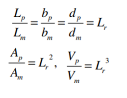
The ratio of all corresponding linear dimension in the model and prototype are equal.

Let Lm = length of model

bm = width of model

dm = diameter of model

Am = area of model

Vm = volume of model

Lp, bp, dp, Ap, Vp are corresponding values of the prototype.

6.8 Similarity

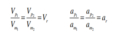
Kinematic Similarity: means the similarity of motion between model and prototype. Thus, kinematic similarity is said to exist between the model and the prototype if the ratios of the velocity and acceleration at the corresponding points in the model and prototype are the same in magnitude; the directions also should be parallel.

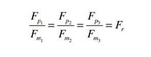
Dynamic Similarity: means the similarity of forces between model and prototype. Thus, dynamic similarity is said to exist between the model and the prototype if the ratios of the forces acting at the corresponding points in the model and prototype are the same in magnitude; the directions also should be parallel.

6.9 Scaling parameters

For the falling-body problem, we select any two of the three parameters to be scaling parameters. Thus we have three options. Let us discuss and display them in turn.

Option 1: Scaling parameters S0 and V0: the effect of gravity g. First use the scaling parameters (S0, V0) to define dimensionless (*) displacement and time. There is only one suitable definition for each:2

Substitute these variables into Eq. and clean everything up until each term is dimensionless. The result is our first option:

This result is shown plotted in Fig. There is a single dimensionless parameter α, which shows here the effect of gravity. It cannot show the direct effects of S0 and V0, since these two are hidden in the ordinate and abscissa. We see that gravity increases the parabolic rate of fall for t* > 0, but not the initial slope at t*= 0. We would learn the same from falling-body data, and the plot, within experimental accuracy, would look like Fig.

Option 2: Scaling parameters V0 and g: the effect of initial displacement S0. Now use the new scaling parameters (V0, g) to define dimensionless (**) displacement and time. Again there is only one suitable definition:

Substitute these variables into Eq. and clean everything up again. The result is our second option:

This result is plotted in Fig. The same single parameter again appears and here shows the effect of initial displacement, which merely moves the curves upward without changing their shape.

Option 3: Scaling parameters S0 and g: the effect of initial speed V0. Finally use the scaling parameters (S0, g) to define dimensionless displacement and time. Again there is only one suitable definition:

Substitute these variables into Eq. and clean everything up as usual. The result is our third and final option:

6.10 Model (or similarity) laws

To ensure dynamic similarity between the model and prototype it is necessary that the ratio of the corresponding forces acting at the corresponding points in the model and prototype be made equal.

It implies that dimensionless numbers should be same for the model as well as the prototype.

This condition is difficult to be satisfied for all the dimensionless numbers.

Hence models are designed on the basis of the force which is dominating in the flow situation. The laws on which the models are designed for dynamic similarity are called model or similarity laws; these are

 Reynolds Model Law

In flow situations where in addition to inertia, viscous force is the other predominant force, the similarity of flow in the model and its prototype can be established if Reynolds number is same for both the systems.

This is known as Reynolds law and according to this law,

Where, ρm = density of fluid in model

Vm = velocity of fluid in model,

Lm = length of linear dimension of the model, and

µm = viscosity of fluid in model

and ρP, VP, LP and µP are the corresponding values of density, velocity, linear dimension and viscosity of fluid in prototype.

[

Following is some of the phenomenon for which Reynolds model law can be a sufficient criterion for similarity of flow in the model and the prototype:

Motion of air planes,

Flow of incompressible fluid in closed pipes,

Motion of submarines completely under water, and

Flow around structures and other bodies immersed completely under moving fluids.

 Froude Model Law

When the gravitational force can be considered to be the only predominant force which controls the motion in addition to the inertia force, the similarity of the flow in any two such systems can be established if the Froude’s number of both the systems is the same.

This is known as Froude’s Model Law.

Some of the phenomenon for which the Froude Model Law can be sufficient criterion for dynamic similarity to be established in the model and the prototype are:

Free surface flows such as flow over spillways, sluices, etc.

Flow of jet from an office or nozzle;

Where waves are likely to be formed on the surface;

Where fluids of different mass densities flow over one another

Let, Vm = velocity of fluid in model

Lm = length (or linear dimension) of the model

gm = acceleration due to gravity (at a place where model is tested)

and VP, LP and gP are the corresponding values of the velocity, length and acceleration due to gravity for the prototype.

Then according to Froude Law,

(Fr)m = (Fr)P

Or ------ 1

As the value of g at the site of mode testing will be practically the same as at site of the proposed prototype, therefore gm = gP and the equation 1 values as

Where Lr = scale ratio for length

6.11 Objectives

1. To obtain information about the likely performance of the prototype

2. To help in the design and to avoid costly mistakes and to evolve an economic solution of a hydraulic problem

6.12 Importance and application of model studies

In recent years, hydraulic model studies are being made in the study and analysis of many problems in fluid mechanics. A hydraulic problem may of course be analyzed by analytical methods, but these analytical methods involve a number of approximations and assumptions and hence their applications often become restricted. In many cases, the analytical methods involve highly complicated equations which cannot be solved.

In spite of the vast progress made in the field of fluid mechanics, the solutions to various complex flow patterns cannot be obtained by analytical methods alone. The available analytical methods need many simplifications so much so that their applications become not only restricted but also theoretical.

There are many cases where it is impossible or impracticable to make a satisfactory and complete mathematical analysis of the problems. A hydraulic model may sometimes provide the only means of ascertaining and eliminating certain undesirable conditions.

It is only through model experiments and research that improvements in the existing works, safe and economic design and construction of new works and furtherance of knowledge on many aspects of hydraulic engineering can be affected.

Model studies are made for two purposes,

i) To obtain information about the likely performance of the prototype, and

(ii) To help in the design and to avoid costly mistakes and to evolve an economic solution of a hydraulic problem.

Applications

model studies have a wide field of applications – dams, rivers and harbours, hydraulic machines, structures, ships, aircraft, seepage problems etc.

i. Dams:

The design of every major dam is checked by model tests before its construction. Besides the model of the dam, all its connected works like spillways, penstocks and gates are studied in order to get detailed information on the flow of water and its effect on the structure. A model study can be helpful in deciding what type of dam may be best suited for any locality and what site can be the best choice for placing a dam.Studies of the models of sluice openings in dams to ascertain the best opening for maximum discharge, studies of various profiles of inlet bell mouths and outlets and studies of the behaviours of gates under operating conditions are of great value. In a penstock where a change of cross-section from a rectangle to a circle for the intake from a dam structure, necessary curves are better decided by model studies.

ii. Rivers and Harbours:

Hydraulic engineers all over the world are involved in considerable amount of work devoted to the dredging of rivers, straightening of channels, protection of banks and bottoms from erosion, various forms of river control and improvement. Harbours and estuaries pose special problems of model design, as it is necessary to duplicate the natural tidal cycles in the model and this may naturally need elaborate machinery.

Model studies can help in studying the wave action of harbours concerned mainly with the effectiveness of the proposed breakwaters for providing protection from waves, and the extent of damage the waves may inflict on the breakwaters. Model studies of breakwater are very essential as there are a number of instances where the breakwaters have failed to provide the adequate protection anticipated of them.

iii. Hydraulic Machines:

Small scale model tests are very useful to obtain performance data for hydraulic turbines and other turbo machines and centrifugal pumps. Model study is a very valuable guide to designers of turbo machines.

iv. Structures:

Where prototype testing is difficult or costly, models provide the proper solution. Many structural tests like deflection tests and destructive and non-destructive testing of structures can be satisfactorily performed on models. Photo elastic and analogy methods of testing of models of dams are very common.

v. Ships:

Towing models in a canal are helpful in estimating Drag force and wave patterns of naval vessels.

vi. Seepage Problems:

It is possible to make studies of seepage flow on geometrically similar sectional models in glass flumes, to find out the uplift pressures on hydraulic structures.

The above are only a few examples of applications of models. It should not be taken for granted that model investigations alone can solve our hydraulic problems. Unless we are able to diagnose the fundamental nature of the problems, the results obtained from the model may be incomplete and may be unreliable. Thus, the correct applicability of model technique is a well-balanced, well studied and well-done combination of model experimentation and analysis.

Analysis involves factors unsolved due to the ignorance of the experiments, which can be solved with the aid of models. Though a well-designed model enables the hydraulic engineer to solve specific problems like those of river control etc., yet the performance is not always a cent percent miniature of the prototypes, because of what can be called model limitations.

It is for this reason that the results obtained from some model experiments are qualitative only. The design, operation and correct interpretation of results, therefore, is a specialised job, requiring quite an amount of experience and good visualisation of the various assumptions made.

Today model analysis has provided the field engineers with a novel tool for studying the various complicated problems and for fixing and regulating the forces of nature to suit his need by properly designed courses.

Numerical

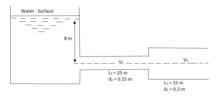
Question: A horizontal pipeline 40 m long is connected to a water tank at one end and discharges freely into the atmosphere to the other end. For first 25 m of its length from the tank, the pipe is 150 mm diameter and diameter are suddenly enlarges to 300 mm. The height of water level in the tank is 8 m above the centre of the pipe. Considering all losses. Find rate of flow. Take f = 0.01 for both pipes.

Given L = 40 m

L1 = 25 m

L2 = 15 m

d1 = 0.15 m

d2 = 0.3 m

H= 8 m

f = 0.01

A1 =

By continuity equation

A1V1 = A2V2

V1 =

Find Q.

Apply Bernoulli’s Theorem to the free surface of water in the tank and outlet of pipe

-------- 1

Hf = Head loss of inlet + Major loss in pipe 1 + Head loss due to sudden enlargement + Major loss in pipe 2

Put in equation 1

Question: A syphon of diameter 200 mm connects two reservoirs having a difference in elevation of 20 m. The length of syphon is 500 m and summit are 3 m above the water level in upper reservoir. The length of the pipe from upper reservoir to the summit is 100 m. Determine the discharge through the syphon. Neglect minor losses. Take f = 0.005 m.

Given

d = 0.2 m

H= 20 m

L = 500 m

h = 3 m

L1 = 100 m

f = 0.005

find Q,

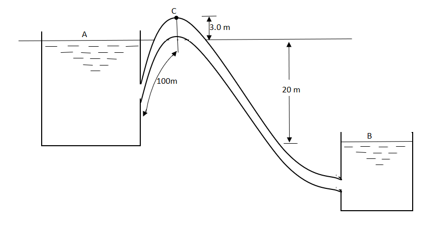
Apply Bernoulli’s equation to point A and B

Apply Bernoulli’s equation to point A and C

Question: A syphon of diameter 200 mm connects two reservoirs having a difference of elevation of 15 m. The total length of the syphon is 600 m and summit are 4m above the water in the upper reservoir. If the separation takes place of 2.8 m water absolute, find max length of syphon from upper reservoir to the summit. Take f = 0.004 and atmospheric pressure = 10.3 m of water

Given

d = 0.2 m

H = 15 m

L = 600 m

h = 4 m

f = 0.004

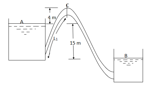
Apply Bernoulli’s equation to point A and B

Apply Bernoulli’s equation to point A and C

Question: Three pipes of 400 mm, 200 mm and 300 mm diameters have lengths of 400 m, 200 m and 300 m are connected in series to join two water tanks having level difference of 16 m. If coefficient of friction is same and equal to 0.005. Determine discharge first neglecting minor losses and the including them

Given

H = 16 m

L1 = 400 m

L2 = 200 m

L3 = 300 m

d1 = 0.4 m

d2 = 0.2 m

d3 = 0.3 m

f1 = f2 = f3 = 0.005

By continuity equation

A1V1 = A2V2

V2 =

Now, Case 1: Neglecting minor losses

Case 2: Minor losses considered

H = Loss at entry + Major loss1 + Loss due to sudden contraction + Major loss 2 + Loss due to sudden enlargement + Major loss 3 + Loss at exit

Question: Three pipes of length 800 m, 500 m and 400 m and of diameters 500 mm, 400 mm, and 300 mm respectively are connected in series. These pipes are to be replaced by a single pipe of length 1700 mm. Find the diameter of the single pipe.

Given

L1 = 800 m

L2 = 500 m

L3 = 400 m

d1 = 0.5 m

d2 = 0.4 m

d3 = 0.3 m

L = 1700 m

Question: A pipeline 0.6 m diameter is 1.5 km long. To increase the discharge, another line of the same diameter is introduced parallel to the first in the second half of the length. Neglecting minor losses, find the increase in discharge if 4f = 0.04. Head at inlet is 300 mm.

D = 0.6 m

l = 1500 m

4f = 0.04

hf = 0.3 m

Case 1: Discharge through single pipe of length 1500 m

Case 2: When additional pipe of length 730 m and diameter 0.6 m connected in parallel with the last half length.

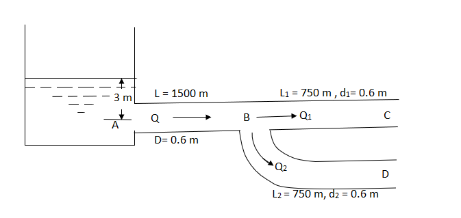
Let Q = Q1 + Q2

But length and diameter of each parallel pipe is same

Consider flow through pipe ABC

-------- 1

Put in equation 1

Increase in discharge = Q – Q’

Question: An old water supply system pipe of 250 mm diameter of a city is to be replaced by two parallel pipes of smaller equal diameter having equal length and identical friction factor values. Find out new diameter required.

D= diameter of each parallel pipes = 0.25 m

Q = Discharge in old pipe

Q1 and Q2 = Discharge in first and second parallel pipe

Hf = hf1 = hf2

Q = Q1 + Q2

As diameter is same for both parallel pipes

But hf = hf1

Question: A 300 mm long pipe line is used for transmission of power. 130kW power is to be transmitted through the pipe in which water having a pressure of 40 bar at inlet is flowing. If pressure drop over the length of pipe is 500kN/m2 and f=0.024. Find i) Diameter of pipe ii) Efficiency of transmission.

Given

L = 3000 m

Power = 130 × 103 watts

P = 40 bar = 40 × 105 N/m2

Pressure drop = 800 kN/m2 = 800 × 103 N/m2

f = 0.024

Question: Using Buckingham’s Πtheorem, show that velocity through circular orifice is given by

Where H= Head causing flow

D = Diameter of orifice

µ = co-efficient of viscosity

ρ = Density

Solution: V is the function of H, D, µ, ρ, and g

Mathematically

Total number of variables n = 6

Writing dimensions of each variable

V = LT-1, H = L, D = L, µ = ML-1T-1, ρ = ML-3, g = LT-2

No. of fundamental dimensions m = 3

No of Π terms = n-m = 6-3 = 3

Each Π term contains (m+1) variables where m=3 and is also equal to repeatingvariables. Choosing H, g, ρ as repeating variables.

For M

For L

For T

and

For M

For L

For T

For M

For L

For T

Substituting the values of in equation 1

Question 2: The discharge Q of a centrifugal pump depends upon the mass density of fluid (ρ), the speed of the pump (N), the diameter of the impeller D, the manometric head Hm and the viscosity of fluid µ. Show that