Unit-4
Probability & Probability distributions
Probability is the study of chances. Probability is the measurement of the degree of uncertainty and therefore, of certainty of the occurrence of events.
Some important definitions-
Random experiment-
An experiment in which all the possible outcomes are known in advance but we cannot predict which of them will occur when we experiment.
Example-‘Throwing a die’ and ‘Drawing a card from a well-shuffled pack of 52 playing cards ‘are examples of a random experiment
Sample space-
Set of all possible outcomes of a random experiment is known as sample space and is usually denoted by S.
Example-
1. If we toss a coin then the sample space is
S = {H, T}, where H and T denote head and tail respectively and n(S) = 2
2. If a coin is tossed thrice or three coins are tossed simultaneously, then the sample space is
S = {HHH, HHT, HTH, THH, HTT, THT, TTH, TTT} and n(S) = 8.
3. If a coin is tossed 4 times or four coins are tossed simultaneously then the sample space is
S = {HHHH, HHHT, HHTH, HTHH, THHH, HHTT, HTHT, HTTH, THHT,
THTH, TTHH, HTTT, THTT, TTHT, TTTH, TTTT} and n(S) = 16.
Sample point-
Each outcome of an experiment is visualized as a sample point in the sample space.
Example- If a die is thrown twice, then getting (1, 1) or (1, 2) or (1, 3) or…or (6, 6) is a sample point.
Event-
A set of one or more possible outcomes of an experiment constitutes what is known as an event. Thus, an event can be defined as a subset of the sample space
Exhaustive cases-
The total number of possible outcomes in a random experiment is called the exhaustive cases
Example-If we throw a die then the number of exhaustive cases is 6 and the sample space, in this case, is {1, 2, 3, 4, 5, 6}
Favourable cases-
The cases which favour the happening of an event are called favourable cases
Example-For the event of getting an even number in throwing a die, the number of favourable cases is 3 and the event, in this case, is {2, 4, 6}.
Mutually exclusive cases-
Cases are said to be mutually exclusive if the happening of any one of them prevents the happening of all others in a single experiment
Equally likely cases-
Two events are said to be ‘equally likely’ if one of them cannot be expected in preference to the other.
Example-if we draw a card from a well-shuffled pack, we may get any card, then the 52 different cases are equally likely.
Odds in favour of an event and odds against an event-
If the number of favourable cases is ‘m’ and the number or not favourable cases are ‘n’.
Then-
1. Odds in favour of the event = m/n
2. Odds against the event = n/m
The classical definition of probability-
Suppose there are ‘n’ exhaustive cases in a random experiment that is equally likely and mutually exclusive.
Let ‘m’ cases are favourable for the happening of an event A, then the probability of happening event A can be defined as-

The probability of non-happening of the event A is defined as-

Note- Always remember that the probability of any events lies between 0 and 1.

Example: A bag contains 7 red and 8 black balls then find the probability of getting a red ball.
Sol.
Here total cases = 7 + 8 = 15
According to the definition of probability,

So that, here favourable cases- red balls = 7
Then,

Addition and multiplication law of probability-
Addition law-
If  are the probabilities of mutually exclusive events, then the probability P, that any of these events will happen is given by
Note-
If two events A and B are not mutually exclusive then the probability of the event that either A or B or both will happen is given by-

Example: A box contains 4 white and 2 black balls and a second box contains three balls of each colour. Now a bag is selected at random and a ball is drawn randomly from the chosen box. Then what will be the probability that the ball is white?
Sol.
Here we have two mutually exclusive cases-
1. The first bag is chosen
2. The second bag is chosen
The chance of choosing the first bag is 1/2. And if this bag is chosen then the probability of drawing a white ball is 4/6.
So that the probability of drawing a white ball from the first bag is-

And the probability of drawing a white ball from the second bag is-

Here the events are mutually exclusive, then the required probability is-

Example-25 lottery tickets are marked with the first 25 numerals. A ticket is drawn at random.
Find the probability that it is a multiple of 5 or 7.
Sol:
Let A be the event that the drawn ticket bears a number multiple of 5 and B be the event that it bears a number multiple of 7.
So that
A = {5, 10, 15, 20, 25}
B = {7, 14, 21}
Here, as A  B =
B =  ,
,
A and B are mutually exclusive
Then,

Multiplication law-
For two events A and B-


Here  is called conditional probability of B given that A has already happened.
Now-
If A and B are two independent events, then-

Because in the case of independent events- 
Example: A bag contains 9 balls, two of which are red three blue, and four black.
Three balls are drawn randomly. What is the probability that-
1. The three balls are of different colours
2. The three balls are of the same colours.
Sol.
1. Three balls will be of a different colour if one ball is red, one blue and one black ball are drawn-
Then the probability will be-

2. Three balls will be of the same colour if one ball is red, one blue and one black ball are drawn-
Then the probability will be-

Example: A die is rolled. If the outcome is a number greater than three. What is the probability that it is a prime number?
Sol.
The sample space is- S = {1, 2, 3, 4, 5, 6}
Let A be the event that an outcome is a number that is greater than three and B be the event that it is a prime.
So that-
A = {4, 5, 6} and B = {2, 3, 5} and hence 
P(A) = 3/6, P(B) = 3/6 and 
Now the required probability-


Example: Two cards are drawn from a pack of playing cards in succession with the replacement of the first card. Find the probability that both are the cards of heart.
Sol.
Let A be the event that the first card drawn is a heart and B be the event that the second card is a heart card.
As the cards are drawn with replacement,
Here A and B are independent and the required probability will be-

Example: Two male and female candidates appear in an interview for two positions in the same post. The probability that the male candidate is selected is 1/7 and the female candidate selected is 1/5.
What is the probability that-
1. Both of them will be selected
2. Only one of them will be selected
3. None of them will be selected.
Sol.
Here, P (male’s selection) = 1/7
And
P (female’s selection) = 1/5
Then-
1.

2.


3.

Example: A can hit a target 3 times in 5 shots, B 2 times in 5 shots, and C 3 times in 4 shots. All of them fire one shot each simultaneously at the target.
What is the probability that-
1. Two shots hit
2. At least two shots hit
Sol.


1. Now probability that 2 shots hit the target-


2.
Probability of at least two shots hitting the target


Let A and B be two events of a sample space Sand let  . Then the conditional probability of the event A, given B, denoted by
 is defined by –

Theorem: If the events AandBdefined on a sample space S of a random experiment are independent, then

Example:A factory has two machines A and B making 60% and 40% respectively of the total production. Machine A produces 3% defective items, and B produces 5% defective items. Find the probability that a given defective part came from A.
SOLUTION:We consider the following events:
A: Selected item comes from A.
B: Selected item comes from B.
D: Selected item is defective.
We are looking for a  . We know:

Now,

So we need


Since D is the union of the mutually exclusive events  and
and  (the entire sample space is the union of the mutually exclusive events A and B)


Example: Two fair dice are rolled, 1 red, and 1 blue. The Sample Space is S = {(1, 1),(1, 2), . . . ,(1, 6), . . . ,(6, 6)}.Total -36 outcomes, all equally likely (here (2, 3) denotes the outcome where the red die show 2 and the blue one shows 3).
(a)Consider the following events:
A: Red die shows 6.
B: Blue die shows 6.
Find ,
,  and
and  .
.
Solution:


NOTE: so
so  for this example. This is not surprising - we expect A to occur in
  of cases. In
  of these cases i.e. in
  of all cases, we expect B to also occur.
(b) Consider the following events:
C: Total Score is 10.
D: Red die shows an even number.
Find  ,
,  and
and  .
.
Solution:


NOTE: so,
so, .
.
Why does multiplication not apply here as in part (a)?
ANSWER: Suppose C occurs: so the outcome is either (4, 6), (5, 5), or (6, 4). In two of these cases, namely (4, 6) and (6, 4), the event D also occurs. Thus
Although , the probability that D occurs given that C occurs is
  .
.
We write , and call
  the conditional probability of D given C.
NOTE: In the above example

Example: Three urns contain 6 red, 4 black; 4 red, 6 black; 5 red, 5 black balls respectively. One of the urns is selected at random and a ball is drawn from it. If the ball is drawn is red find the probability that it is drawn from the first urn.
Solution:
 :The ball is drawn from urnI.
 : The ball is drawn from urnII.
 : The ball is drawn from urnIII.
R:The ball is red.
We have to find 

Since the three urns are equally likely to be selected

Also,


From (i), we have

Key takeaways-


5. 
Let S be a sample space and  be n mutually exclusive events with P(
 .
.
Let A be an event which is a sub-set of  with P(A)>0, then-

Where i = 1, 2, ……. ,n
And  [which is the law of total probability]
Example- Three urn contains 6 red, 4 black; 4 red, 6 black; 5 red, 5 black balls respectively. One of the urn is selected randomly and a ball is drawn from it.
If the ball drawn is red then find the probability that it is drawn from the first urn.
Sol.
Let,


Now we have to find- 
By using Bayes theorem-
 =
= 
Here three urns equally likely to be selected-
So that-

And-


So that-
 =
= 
Hence the required probability is 2/5.
Example: A person speaks the truth 3 out of 4 times. A die is thrown. She reports that there are five. What is the chance there is 5?
Sol.
Let  be the event that the person speaksthe truth,
  be the event that she tells lie and A be the event that she reports a five.
So that-
By the law of total probability-


Now we have to find- 
By using Bayes theorem-
 =
= 
 =
= 
Which is the required probability.
Example: ln a bolt factory machines  and
and  manufacturerespectively 25%, 35% and 40% of the total. lf their output 5, 4, and 2 percent are defective bolts. A bolt is drawn at random from theproduct and is found to be defective. What is the probability that it was manufactured by machine B.?
Solution: bolt is manufactured by machine 
 : bolt is manufactured by machine
 : bolt is manufactured by machine

The probability of drawing a defective bolt manufactured by machine  is
is  (D/A)
(D/A) 
Similarly,  (D/B)
(D/B)  and
and  (D/C)
(D/C) 
By Baye’s theorem


Key takeaways-

A random variable is a real-valued function whose domain is a set of possible outcomes of a random experiment and range is a subset of the set of real numbers and has the following properties:
i) Each particular value of the random variable can be assigned some probability
ii) Uniting all the probabilities associated with all the different values of the random variable gives the value 1.
A random variable is denoted by X, Y, Z, etc.
For example, if a random experiment E consists of tossing a pair of dice, the sum X of the two numbers which turn up have the value 2,3,4,…12 depending on chance. Then X is a random variable
Discrete random variable-
A random variable is said to be discrete if it has either a finite or a countable number of values. A countable number of values means the values which can be arranged in a sequence.
Note- if a random variable takes a finite set of values it is called discrete and if a random variable takes an infinite number of uncountable values it is called a continuous variable.
By definition, a random variable X and its distribution are discrete if X assumes only finitely many or at most countably many values  called the possible values of X. with positive probabilities
  is zero for any interval J containing no possible values.
The discrete distribution of X is also determined by the probability functions f (x) of X, defined by

From this, we get the values of the distribution function F (x) by taking sums.

Example: 1. No. of head obtained when two coins are tossed.
2. No. of defective items in a lot.
Discrete probability distributions-
Let X be a discrete variate which is the outcome of some experiments. If the probability that X takes the values of x is  , then-

Where-
1. 
2. 
The set of values  with their probabilities
  makes a discrete probability distribution of the discrete random variable X.
The probability distribution of a random variable X can be exhibited as follows-
X |
|
|
|
P(x) |
|
|
|
Example: Find the probability distribution of the number of heads when three coins are tossed simultaneously.
Sol.
Let be the number of heads in the toss of three coints
The sample space will be-
{HHH, HHT, HTH, THH, HTT, THT, TTH, TTT}
Here variable X can take the values 0, 1, 2, 3 with the following probabilities-
P[X= 0] = P[TTT] = 1/8
P[X = 1] = P [HTT, THH, TTH] = 3/8
P[X = 2] = P[HHT, HTH, THH] = 3/8
P[X = 3] = P[HHH] = 1/8
Hence the probability distribution of X will be-
X |
|
|
|
|
P(x) |
|
|
|
|
Example: For the following probability distribution of a discrete random variable X,

Find-
1. The value of c.
2. P[1<x<4]
Sol,
1. We know that-

So that-
0 + c + c + 2c + 3c + c = 1
8c = 1
Then c = 1/8
Now, 2. P[1<x<4] = P[X = 2] + P[X = 3] = c + 2c = 3c = 3× 1/8 = 3/8
Let a random variable X has a probability distribution which assumes the values say with their associated probabilities
  then the mathematical expectation can be defined as-

The expected value of a random variable X is written as E(X).
The expected value for a continuous random variable is

The mean value (μ) of the probability distribution of a variate X is commonly known as its expectation current is denoted by E (X). If f(x) is the probability density function of the variate X, then
 (discrete distribution)
 (continuous distribution)
In general expectation of any function is  given by
 (discrete distribution)
 (continuous distribution)
(2) Variance offer distribution is given by
 (discrete distribution)
 (continuous distribution)
Where  is the standard deviation of the distribution.
(3) The rth moment about mean (denoted by  is defined by
 (discrete function)
 (continuous function)
(4) Mean deviation from the mean is given by
 (discrete distribution)
 (continuous distribution)
Example: If a random variable X has the following probability distribution in the tabular form then what will be the expected value of X.
X | 0 | 1 | 2 |
P(x) | 1/4 | ½ | ¼ |
Sol.
We know that-

So that-

Example: Find the expectations of the number of an unbiased die when thrown.
Sol. Let X be a random variable that represents the number on a die when thrown.
X can take the values-
1, 2, 3, 4, 5, 6
With
P[X = 1] = P[X = 2] = P[ X = 3] = P[X = 4] = P[X = 5] = P[X = 6] = 1/6
The distribution table will be-
X | 1 | 2 | 3 | 4 | 5 | 6 |
p(x) | 1/6 | 1/6 | 1/6 | 1/6 | 1/6 | 1/6 |
Hence the expectation of number on the die thrown is-

So that-

Example. In a lottery, m tickets are drawn at a time out of a ticket numbered from 1 to n. Find the expected value of the sum of the numbers on the tickets drawn.
Solution. Let  be the variables representing the numbers on the first, second,…nth ticket. The probability of drawing a ticket out of n ticket spelling in each case 1/n, we have

Therefore the expected value of the sum of the numbers on the tickets drawn


Example. X is a continuous random variable with probability density function given by


Find k and mean value of X.
Solution. Since the total probability is unity.


Mean of X =


Example. The frequency distribution of a measurable characteristic varying between 0 and 2 is as under


Calculate two standard deviation and also the mean deviation about the mean.
Solution. Total frequency N =
 (about the origin)=

 (about the origin)=


Hence, 
i.e., standard deviation 
Mean derivation about the mean


A probability distribution is an arithmetical function that defines completely possible values &possibilities that a random variable can take in a given range. This range will be bounded between the minimum and maximum possible values. But exactly where the possible value is possible to be plotted on the probability distribution depends on some influences. These factors include the distribution's mean, SD, Skewness, and kurtosis.
Binomial Distribution:
Binomial Distribution 

To find the probability of the happening of an event once, twice, …., r times… exactly in n trials.
Let the probability of the happening of an event A in one trial be  and its probability of not happening be
We assume that there are n trials and the happening of the event  is
is times and it’s not happening n-r times.
This may be shown as follows


 times
times  times …. (1)
A indicates it's happening,  its failure, and
 .
.
We see that (1) has the probability
 …. (2)
r times n-r times
Clearly (1) is merely one order of arranging r A’s
The probability of (1) Number of different arrangements of
  and
and  .
.
The number of different arrangements of  and
and 
 Probability off the happening of an event
  times
times 
 th term of

If  , probability of happening of an event 0 times
If  , probability of happening of an event 1 time
If  , probability of happening of an event 2 times
If  , probability of happening of an event 3 times
These terms are the successive terms in the expansion of  . Hence it is called Binomial distribution.
Example
If on average one ship in every ten is wrecked, find the probability that of 5 ships expected to arrive, 4 at least will arrive safely.
Solution:
Out of 10 ships, one ship is wrecked.
i.e., Nine ships out of ten ships are safe. P(safety)
P(At least 4 ships out of 5 ships are safe)

Example
The overall percentage of failures in a certain examination is 20. If six candidates appear in the examination, what is the probability that at least five pass the examination?
Solution:
Probability of failures 

Probability 
Probability of at least five passes  P(5 or 6)


Example
The probability that a managed 60 will live to be 70 is 0.65. What is the probability that out of 10 items, now 60, at least 7 will live to be 70?
Solution
The probability that a man aged 60 will live to be 70


Number of men
The probability that at least 7 men will live to


Example
A die is thrown 8 times and it is required to find the probability that 3 will show (i) Exactly 2 times
(ii) At least seven times (iii) At least once.
Solution:
The probability of throwing 3 in a single trial =
The probability of not throwing 3 in a single trial 
(i) P (getting 3 exactly 2 times) =P (getting 3, at 7 or 8 times) 
(ii) P (getting 3, at least seven times) =P (getting 3, at 7 or 8 times) 
(iii) P (getting 3 at least once)
=P (getting 4, at 1 or 2 or 3 or 4 or 5 or 6 or 7 or 8 times)

Example:
Assuming that 20% of the population of a city are literate, so that the chance of an individual being literate is  and assuming that 100 investigators each take 10 individuals to see whether they are literate, how many investigators would you expect 3 or less were literate.
Solution 

P (3 or less) = P (0 or 1 or 2 or 3 )

Required number of investigators
 approximately
Mean of Binomial Distribution

Successes | Frequency |
|
0 |
|
|
1 |
|
|
2 |
|
|
3 |
|
|
… | …. | …. |
4 |
|
|


Hence Mean
Standard Deviation of Binomial Distribution
Successes | Frequency |
|
0 |
|
|
1 |
|
|
2 |
|
|
3 |
|
|
…. | …. | … |
N |
|
|
We know that  ….(1)
….(1)
 is the deviation of items (successes) from 0.


Putting these values in (1), we have
Variance

Hence for the binomial distribution, Mean
Example:
A die is tossed thrice. Success is getting 1 or 6 on a toss. Find the mean and variance of the number of successes.
Solution:

Mean
Variance
Recurrence relation for the binomial distribution
By Binomial distribution 

On dividing (2) by (1), we get

Poisson Distribution:
Poisson distribution is a particular limiting form of the Binomial distribution when p or (q) is very small and n is large enough.
Poisson distribution is 
Where m is the mean of the distribution.
Proof:
In Binomial distribution
 { Since mean
 }
}
 (
( is constant)


Taking limits, when n tends to infinity


Mean of Poisson Distribution

Successes | Frequency |
|
0 |
| 0 |
1 |
|
|
2 |
|
|
3 |
|
|
… | … | …. |
R |
|
|
… | … | …. |


Mean

Standard Deviation of Poisson Distribution

Successes | Frequency | Product | Product |
0 |
| 0
| 0 |
1 |
|
|
|
2 |
|
|
|
3 |
|
|
|
… | …. | …. | … |
R |
|
|
|
… | …. | … | … |


Hence mean and variance of a Poisson distribution are each equal to m. Similarly, we can obtain,


Mean Deviation:
Show that in a Poisson distribution with unit mean, and the mean deviation about the mean is  times the standard deviation.
Solution: But mean=1 i.e.,
  and
and 
Hence, 
|
|
|
|
0 |
| 1 |
|
1 |
| 0 |
|
2 |
| 1 |
|
3 |
| 2 |
|
4 |
| 4 |
|
… | …. | …. | … |
R |
| r-1 |
|
Mean Derivation


Moment Generating Function of Poisson Distribution

Solution:
Let be the moment generating function, then

Cumulants
The cumulant generating function  is given by


Now  cumulant
 Coefficient of
  in K(t)
i.e.,  where
where 
Mean 


Recurrence formula for Poisson Distribution:
Solution: Poisson Distribution


On dividing (2) by (1) we get


Example
Assume that the probability of an individual coal miner being killed in a mine accident during a year is . Use appropriate statistical distribution to calculate the probability that in a mine employing 200 metres, there will be at least one fatal accident in a year.
Solution:
 ,
, 

P(At least one)=P(1 or 2 or 3 or …. or 200)

Example:
Suppose 3% of bolts made by a machine are defective, the defects occurring at random during production. If bolts are packaged 50 per box, find
(a) exact probability and
(b) Poisson approximation to it, that a given box will contain 5 defectives.
Solution:


(a) Hence the probability for 5 defective bolts in a lot of 50
 (Binomial Distribution)
(b) To get Poisson approximation 
Required Poisson approximation
Example:
In a certain factory producing cycle tyres there is a small chance of 1 in 500 tyres to be defective. The tyres are supplied in lots of 10. Using Poisson distribution calculate the approximate number of lots containing no defective, one defective, and two defective tyres, respectively, in a consignment of 10000 lots.
Solution:


S.No | Probability of defective | Number of lots containing defective |
1 |
|
|
2 |
|
|
3 |
|
|
Normal Distribution:
The normal distribution is continuous. It is derived as the limiting form of the Binomial distribution for large values of n and p and q are not very small.
The Normal distribution is given by the equation
 ….(1)
….(1)
Where  mean,
mean,  standard deviation,
  ,
, 

On substitution  in (1), we get
 ….(2)
….(2)
Here mean , standard deviation
(2) is known as the standard form of normal distribution.
Mean for Normal Distribution:
Mean [Putting
  ]
]


Standard Deviation for Normal Distribution:

Put 


Median of the Normal Distribution
If a is the median, then it divides the total area into two halves so that,

Where 
Suppose mean,
mean,  then
then
 [But
[But ]
]
 (
( mean)
mean)

Thus 
Similarly, when  mean, we have
Thus, median=median .
.
Mean Deviation about the Mean
Mean Deviation 

 where
where

 (as the function is given)
 approximately.
Mode of the Normal distribution
We know that mode is the value of the variate x for which  is maximum. Thus, differential calculus
  is maximum if
  and
and 
Where 
Clearly will be maximum when the exponent will bemaximum which will be the when
Thus mode is  and modal ordinate
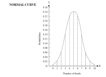
Let us show binomial distribution graphically. The probabilities of heads in 1 toss are
 .
.
 . It is shown in the given figure.
If the variates (heads here) are treated as if they were continuous, the required probability curve will be normal as shown in the above figure by dotted lines.
Properties of the normal curve:


(b) 
(c) 
Hence (a) About  of the values will lie between
  and
and  .
.
(b) About 95% of the values will lie between and
and  .
.
(c) About 99.7% of the values will lie between and
and  .
.
The area under the Normal curve
By taking  , the standard normal curve is formed.
The total area under this curve is 1. The area under the curve is divided into two equal parts . The left-hand side is and right-hand side area too
  is
is  . The area between the ordinate
 .
.
Example
On final examination in mathematics, the mean was 72, and the standard deviation was 15. Determine the standard deviation scores of students receiving grades.
(a) 60 (b) 93 (c) 72
Solution:
(a)  (b)
(b)  (c)
(c) 
Example: Find the area under the normal curve in each of the cases.


Solution:
(a) Area between  and
and  (b) Area between
  and
and 


(c) Required area  (Area between
  and
and  )+
)+
(Area between  and
and  )
)
=(Area between  and
and  )
)
+(Area between  and
and  )
)

(d) Required area  (Area between
  and
and  ) – (Area between
  and
and  )
)
(e) Required area (Area between
  and
and  )
)

(f) Required area = (Area between  and
and  )
)


Example. The mean inside diameter of a sample of 200 washers produced by a machine is 0.0502 cm and the standard derivation is 0.005 cm. The purpose for which these washers are intended allows a maximum tolerance in the diameter of 0.496 to 0.508 cm, otherwise, the washers are considered defective. Determine the percentage of defective washers produced by the machine, assuming the diameters are normally distributed
Solution:


Area for non-defective washers Area between
  and
and 
= 2 Area between  and
and 

Percentage of defective washers

Example:
A manufacturer knows from experience that the resistance of resistors he produces is normal with mean  and standard deviation
  What percentage of resistors will have resistance between 98 ohms and 102 ohms?
Solution:


Area between  and
and 
 (Area between
  and
and  )+(Area between
  and
and  )
)
 (Area between
  and
and  )=2
)=2 0.3413=0.6826
Percentage of resistors having resistance between 98 ohms and 102 ohms =68.26
Example
In a normal distribution, 31% of the items are under 45 and 8% are over 64. Find the mean and standard deviation of the distribution.
Solution:
Let  be the mean and
  S.D.
S.D.
If 
If 
The area between 0 and 
[From the table, for the area  ]
]
 …(1)
…(1)
The area between  and
and 
(From the table, for the area )
)
 …(2)
…(2)
Solving (1) and (2), we get
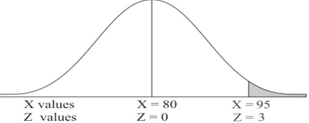
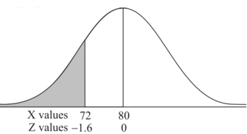
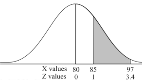
Example: If a random variable X is normally distributed with mean 80 and standard deviation 5, then find-
1. P[X > 95]
2. P[X < 72]
3. P [85 < X <97]
[Note- use the table- area under the normal curve]
Sol.
The standard normal variate is – 
Now-
1. X = 95,

So that-


2. X = 72,

So that-


3. X = 85,

X = 97,

So that-


Example: In a company, the mean weight of 1000 employees is 60kg and the standard deviation is 16kg.
Find the number of employees having their weights-
1. Less than 55kg.
2. More than 70kg.
3. Between 45kg and 65kg.
Sol. Suppose X be a normal variate = the weight of employees.
Here mean 60kg and S.D. = 16kg
X 
Then we know that-

We get from the data,

Now-
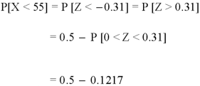
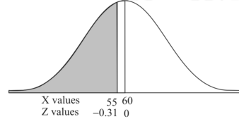
1. For X = 55,

So that-

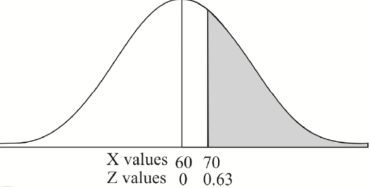
2. For X = 70,

So that-


3. For X = 45,

For X = 65,


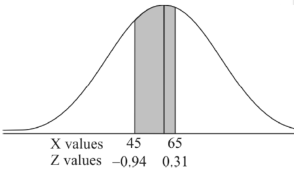
Hence the number of employees having weights between 45kg and 65kg-

Example: The life of electric bulbs is normally distributed with a mean of 8 months and a standard deviation of 2 months.
If 5000 electric bulbs are issued how many bulbs should be expected to need replacement after 12 months?
[Given that P (z ≥ 2) = 0. 0228]
Sol.
Here mean (μ) = 8 and standard deviation = 2
Number of bulbs = 5000
Total months (X) = 12
We know that-

Area (z ≥ 2) = 0.0228
Number of electric bulbs whose life is more than 12 months ( Z> 12)
= 5000 × 0.0228 = 114
Therefore replacement after 12 months = 5000 – 114 = 4886 electric bulbs.
Key takeaways-


4. The Normal distribution is given by the equation

5. median=median in case of normal distribution
Population-
The population is the collection or group of observations under study.
The total number of observations in a population is known as population size and it is denoted by N.
Types of population-
Sample –
To get the information from all the elements of a large population may be time consuming and difficult. And also if the elements of population are destroyed under investigation then getting the information from all the units is not make a sense. For example, to test the blood, doctors take very small amount of blood. Or to test the quality of certain sweet we take a small piece of sweet In such situations, a small part of population is selected from the population which is called a sample
Complete survey-
When each and every element of the population is investigated or studied for the characteristics under study then we call it complete survey or census.
Sample Survey-
When only a part or a small number of elements of population are investigated or studied for the characteristics under study then we call it sample survey or sample enumeration Simple Random Sampling or Random Sampling
The simplest and most common method of sampling is simple random sampling. In simple random sampling, the sample is drawn in such a way that each element or unit of the population has an equal and independent chance of being included in the sample. If a sample is drawn by this method then it is known as a simple random sample or random sample
Simple Random Sampling without Replacement (SRSWOR)
In simple random sampling, if the elements or units are selected or drawn one by one in such a way that an element or unit drawn at a time is not replaced back to the population before the subsequent draws is called SRSWOR.
Suppose we draw a sample from a population, the size of sample is n and the size of population is N, then total number of possible sample is 
Simple Random Sampling with Replacement (SRSWR)
In simple random sampling, if the elements or units are selected or drawn one by one in such a way that a unit drawn at a time is replaced back to the population before the subsequent draw is called SRSWR.
Suppose we draw a sample from a population, the size of sample is n and the size of population is N, then total number of possible samples is  .
.
Parameter-
A parameter is a function of population values which is used to represent the certain characteristic of the population. For example, population mean, population variance, population coefficient of variation, population correlation coefficient, etc. are all parameters. Population parameter mean usually denoted by μ and population variance denoted by 
Sample mean and sample variance-
Let  be a random sample of size n taken from a population whose pmf or pdf function f(x,
Then the sample mean is defined by-

And sample variance-

Statistic-
Any quantity which does not contain any unknown parameter and calculated from sample values is known as statistic.
Suppose  is a random sample of size n taken from a population with mean μ and variance
  then the sample mean-

Is a statistic.
Estimator and estimate-
if a statistic is used to estimate an unknown population parameter then it is known as estimator and the value of the estimator based on observed value of the sample is known as estimate of parameter.
Hypothesis-
A hypothesis is a statement or a claim or an assumption about the value of a population parameter.
Similarly, in case of two or more populations a hypothesis is comparative statement or a claim or an assumption about the values of population parameters.
For example-
If a customer of a car wants to test whether the claim of car of a certain brand gives the average of 30km/hr is true or false.
Simple and composite hypotheses-
If a hypothesis specifies only one value or exact value of the population parameter then it is known as simple hypothesis. And if a hypothesis specifies not just one value but a range of values that the population parameter may assume is called a composite hypothesis.
Null and alternative hypothesis
The hypothesis which is to be tested as called the null hypothesis.
The hypothesis which complements to the null hypothesis is called alternative hypothesis.
In the example of car, the claim is  and its complement is
  .
.
The null and alternative hypothesis can be formulated as-

And

Example: A company has replaced its original technology of producing electric bulbs with CFL technology. The company manager wants to compare the average life of bulbs manufactured by original technology and new technology CFL. Write appropriate null and alternate hypotheses
Sol.
Let the average life of original and CFL technology bulbs are denoted by  and
and  .
.
The null and alternative hypotheses will be-


Here the alternate hypothesis is two-tailed so that the test will also be two-tailed.
If the manager is interested just to know whether the average life of CFL is greater than the original technology bulbs then the null and alternative hypotheses will be-


Here the alternative hypothesis is left tailed so that the corresponding test will also be left tailed.
Critical region-
Let  be a random sample drawn from a population having unknown population parameter
  .
.
The collection of all possible values of  is called sample space and a particular value represent a point in that space.
In order to test a hypothesis, the entire sample space is partitioned into two disjoint sub-spaces, say,  and S –
  . If calculated value of the test statistic lies in , then we reject the null hypothesis and if it lies in
  then we do not reject the null hypothesis. The region is called a “rejection region or critical region” and the region
  is called a “non-rejection region”.
Therefore, we can say that
“A region in the sample space in which if the calculated value of the test statistic lies, we reject the null hypothesis then it is called critical region or rejection region.”
The region of rejection is called critical region.
The critical region lies in one or two tails on the probability curve of sampling distribution of the test statistic it depends on the alternative hypothesis.
Therefore there are three cases-
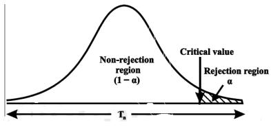
CASE-1: if the alternative hypothesis is right sided such as  then the entire critical region of size
  lies on right tail of the probability curve.
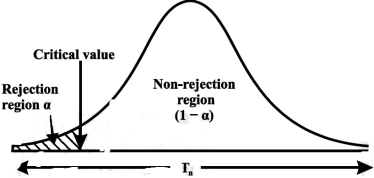
CASE-2: if the alternative hypothesis is left sided such as  then the entire critical region of size
  lies on left tail of the probability curve.
CASE-3: if the alternative hypothesis is two sided such as  then the entire critical region of size
  lies on both tail of the probability curve
Type-1 and Type-2 error-
Type-1 error-
The decision relating to rejection of null hypo. When it is true is called type-1 error.
The probability of type-1 error is called size of the test, it is denoted by  and defined as-

Note-
 is the probability of correct decision.
Type-2 error-
The decision relating to non-rejection of null hypo. When it is false is called type-1 error.
It is denoted by  and defined as-

Decision | |
|
Reject | Type-1 error | Correct decision |
Do not reject | Correct decision | Type-2 error |
One tailed and two tailed tests-
A test of testing the null hypothesis is said to be two-tailed test if the alternative hypothesis is two-tailed whereas if the alternative hypothesis is one-tailed then a test of testing the null hypothesis is said to be one-tailed test.
For example, if our null and alternative hypothesis are-

then the test for testing the null hypothesis is two-tailed test because the
alternative hypothesis is two-tailed.
If the null and alternative hypotheses are-

then the test for testing the null hypothesis is right-tailed test because the alternative hypothesis is right-tailed.
Similarly, if the null and alternative hypotheses are-

then the test for testing the null hypothesis is left-tailed test because the alternative hypothesis is left-tailed
Procedure for testing a hypothesis-
Step-1: first we set up null hypothesis  and alternative hypothesis
  .
.
Step-2: after setting the null and alternative hypothesis, we establish a
criteria for rejection or non-rejection of null hypothesis, that is,
decide the level of significance ( ), at which we want to test our
hypothesis. Generally, it is taken as 5% or 1% (α = 0.05 or 0.01).
step-3: The third step is to choose an appropriate test statistic under H0 for
testing the null hypothesis as given below

Now after doing this, specify the sampling distribution of the test statistic preferably in the standard form like Z (standard normal),  , t, F or any other well-known in literature
Step-4: Calculate the value of the test statistic described in Step III on the basis of observed sample observations.
Step-5: Obtain the critical (or cut-off) value(s) in the sampling distribution of the test statistic and construct rejection (critical) region of size  .
.
Generally, critical values for various levels of significance are putted in the form of a table for various standard sampling distributions of test statistic such as Z-table,  -table, t-table, etc
Step-6: After that, compare the calculated value of test statistic obtained from Step IV, with the critical value(s) obtained in Step V and locates the position of the calculated test statistic, that is, it lies in rejection region or non-rejection region.
Step-7: in testing the hypothesis we have to reach at a conclusion, it is performed as below-
First- If calculated value of test statistic lies in rejection region at  level of significance then we reject null hypothesis. It means that the sample data provide us sufficient evidence against the null hypothesis and there is a significant difference between hypothesized value and observed value of the parameter
Second- If calculated value of test statistic lies in non-rejection region at  level of significance then we do not reject null hypothesis. Its means that the sample data fails to provide us sufficient evidence against the null hypothesis and the difference between hypothesized value and observed value of the parameter due to fluctuation of sample
Procedure of testing of hypothesis for large samples-
The sample size more than 30 is considered as large sample size. So that for large samples, we follow the following procedure to test the hypothesis.
Step-1: first we set up the null and alternative hypothesis.
Step-2: After setting the null and alternative hypotheses, we have to choose level of significance. Generally, it is taken as 5% or 1% (α = 0.05 or 0.01). And accordingly rejection and non-rejection regions will be decided.
Step-3: Third step is to determine an appropriate test statistic, say, Z in case of large samples. Suppose Tn is the sample statistic such as sample
mean, sample proportion, sample variance, etc. for the parameter 
then for testing the null hypothesis, test statistic is given by

Step-4: the test statistic Z will be assumed to be approximately normally distributed with mean 0 and variance 1 as

By putting the values in above formula, we calculate test statistic Z.
Suppose z be the calculated value of Z statistic
Step-5: After that, we obtain the critical (cut-off or tabulated) value(s) in the sampling distribution of the test statistic Z corresponding to  assumed in Step II. we construct rejection (critical) region of size α in the probability curve of the sampling distribution of test statistic Z.
Step-6: Take the decision about the null hypothesis based on the calculated and critical values of test statistic obtained in Step IV and Step V.
Since critical value depends upon the nature of the test that it is one tailed test or two-tailed test so following cases arise-
Case-1 one-tailed test- when  (right-tailed test)
In this case, the rejection (critical) region falls under the right tail of the probability curve of the sampling distribution of test statistic Z.
Suppose  is the critical value at
  level of significance so entire region greater than or equal to
  is the rejection region and less than
 is the non-rejection region
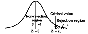
If z (calculated value ) ≥  (tabulated value), that means the calculated value of test statistic Z lies in the rejection region, then we reject the null hypothesis H0 at
  level of significance. Therefore, we conclude that sample data provides us sufficient evidence against the null hypothesis and there is a significant difference between hypothesized or specified value and observed value of the parameter.
If z < that means the calculated value of test statistic Z lies in non rejection region, then we do not reject the null hypothesis H0 at
  level of significance. Therefore, we conclude that the sample data fails to provide us sufficient evidence against the null hypothesis and the difference between hypothesized value and observed value of the parameter due to fluctuation of sample.
So the population parameter 
Case-2: when  (left-tailed test)
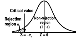
the rejection (critical) region falls under the left tail of the probability curve of the sampling distribution of test statistic Z.
Suppose - is the critical value at
  level of significance then entire region less than or equal to -
 is the rejection region and greater than -
 is the non-rejection region
If z ≤- , that means the calculated value of test statistic Z lies in the rejection region, then we reject the null hypothesis H0 at
  level of significance.
If z >- , that means the calculated value of test statistic Z lies in the non-rejection region, then we do not reject the null hypothesis H0 at
  level of significance.
In case of two tailed test-

In this case, the rejection region falls under both tails of the probability curve of sampling distribution of the test statistic Z. Half the area (α) i.e. α/2 will lies under left tail and other half under the right tail. Suppose  and
and  are the two critical values at the left-tailed and right-tailed respectively. Therefore, entire region less than or equal to
  and greater than or equal to
  are the rejection regions and between -
 is the non-rejection region.
If Z that means the calculated value of test statistic Z lies in the rejection region, then we reject the null hypothesis H0 at
  level of significance.
If  that means the calculated value of test statistic Z lies in the non-rejection region, then we do not reject the null hypothesis H0 at
  level of significance.
Testing of hypothesis for population mean using Z-Test
For testing the null hypothesis, the test statistic Z is given as-

The sampling distribution of the test statistics depends upon variance 
So that there are two cases-
Case-1: when  is known -
The test statistic follows the normal distribution with mean 0 and variance unity when the sample size is the large as the population under study is normal or non-normal. If the sample size is small then test statistic Z follows the normal distribution only when population under study is normal. Thus,

Case-1: when  is unknown –
We estimate the value of  by using the value of sample variance

Then the test statistic becomes-

After that, we calculate the value of test statistic as may be the case ( is known or unknown) and compare it with the critical value at prefixed level of significance α.
Example: A company of pens claims that a certain pen manufactured by him has a mean writing-life at least 460 A-4 size pages. A purchasing agent selects a sample of 100 pens and put them on the test. The mean writing-life of the sample found 453 A-4 size pages with standard deviation 25 A-4 size pages. Should the purchasing agent reject the manufacturer’s claim at 1% level of significance?
Sol.
It is given that-
Specified value of population mean =  = 460,
Sample size = 100
Sample mean = 453
Sample standard deviation = S = 25
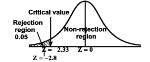
The null and alternative hypothesis will be-

Also the alternative hypothesis left-tailed so that the test is left tailed test.
Here, we want to test the hypothesis regarding population mean when population SD is unknown. So we should used t-test for if writing-life of pen follows normal distribution. But it is not the case. Since sample size is n = 100 (n > 30) large so we go for Z-test. The test statistic of Z-test is given by


We get the critical value of left tailed Z test at 1% level of significance is 
Since calculated value of test statistic Z (= ‒2.8) is less than the critical value
(= −2.33), that means calculated value of test statistic Z lies in rejection region so we reject the null hypothesis. Since the null hypothesis is the claim so we reject the manufacturer’s claim at 1% level of significance.
Example: A big company uses thousands of CFL lights every year. The brand that the company has been using in the past has average life of 1200 hours. A new brand is offered to the company at a price lower than they are paying for the old brand. Consequently, a sample of 100 CFL light of new brand is tested which yields an average life of 1220 hours with standard deviation 90 hours. Should the company accept the new brand at 5% level of significance?
Sol.
Here we have-

The company may accept the new CFL light when average life of
CFL light is greater than 1200 hours. So the company wants to test that the new brand CFL light has an average life greater than 1200 hours. So our claim is  > 1200 and its complement is
  ≤ 1200. Since complement contains the equality sign so we can take the complement as the null hypothesis and the claim as the alternative hypothesis. Thus,

Since the alternative hypothesis is right-tailed so the test is right-tailed test.
Here, we want to test the hypothesis regarding population mean when population SD is unknown, so we should use t-test if the distribution of life of bulbs known to be normal. But it is not the case. Since the sample size is large (n > 30) so we can go for Z-test instead of t-test.
Therefore, test statistic is given by


The critical values for right-tailed test at 5% level of significance is
 1.645
1.645
Since calculated value of test statistic Z (= 2.22) is greater than critical value (= 1.645), that means it lies in rejection region so we reject the null hypothesis and support the alternative hypothesis i.e. we support our claim at 5% level of significance
Thus, we conclude that sample does not provide us sufficient evidence against the claim so we may assume that the company accepts the new brand of bulbs
Example: A manufacturer of electric bulbs claims that a certain pen manufactured by him has a mean life of at least 460 days. A purchasing officer selects a sample of 100 bulbs and put them on the test. The mean life of the sample found 453 days with a standard deviation of 25 days. Should the purchasing officer reject the manufacturer’s claim at a 1% level of significance?
Sol.
Here the population mean = 
Sample size = n = 100
Sample mean = 
Sample standard deviation = S = 25
The null and alternative hypotheses will be-

Here alternative hypothesis is left tailed so that the test is left tailed test-
Here population standard deviation is unknown so that we should use a t-test if the life of the bulbs follows a normal distribution.
But it is not the case. Here sample size is 100 which is large.
Note- a sample size of more than 30 is considered a large sample.
So here we use Z-test-


The critical value of Z statistic at a 1% level of significance is = -2.33
Since the calculated value of the test statistic is less than the critical value that means the test statistic lies in the rejection region.
Therefore we reject the null hypothesis.
So that we reject the manufacturer’s claim at a 1% level of significance.
Level of significance-
The probability of type-1 error is called level of significance of a test. It is also called the size of the test or size of the critical region. Denoted by  .
.
Basically it is prefixed as 5% or 1% level of significance.
If the calculated value of the test statistics lies in the critical region then we reject the null hypothesis.
The level of significance relates to the trueness of the conclusion. If null hypothesis do not reject at level 5% then a person will be sure “concluding about the null hypothesis” is true with 95% assurance but even it may false with 5% chance.
Confidence limits-
Let  be a random sample of size n drawn from a population having pdf (pmf)
  .
.
Let  and
and  (here
(here  be two statistic such that the probability that the random interval [
 ] including the true value of population parameter
  , that is-

Here  does not depends on
  .
.
Then the random interval [ ] is called as (1 –
  100 % confidence interval for unknown population parameter
  and (1 –
  is known as confidence coefficient.
The length of interval can be defined as-
Length = Upper confidence – Lower confidence limit
The chi-square test works under the following circumstances-
1. When the given data is normally distributed.
2. Sample observations are random and independent.
When a fair coin is tossed 80 times we expect from the theoretical considerations that heads will appear 40 times and tail 40 times. But this never happens in practice that is the results obtained in an experiment do not agree exactly with the theoretical results. The magnitude of discrepancy between observations and theory is given by the quantity  (pronounced as chi-squares). If
  the observed and theoretical frequencies completely agree. As the value of
  increases, the discrepancy between the observed and theoretical frequencies increases.
(1) Definition. If  and
and  be the corresponding set of expected (theoretical) frequencies, then
  is defined by the relation


(2) Chi-square distribution
If  be n independent normal variates with mean zero and s.d. unity, then it can be shown that
  is a random variate having
  distribution with ndf.
The equation of the  curve is

(3) Properties of  distribution


 have been tabulated for various values of P and for values of v from 1 to 30. (Table V Appendix 2)
 ,the
,the curve approximates to the normal curve and we should refer to normal distribution tables for significant values of
  .
.
IV. Since the equation of  the curve does not involve any parameters of the population, this distribution does not dependent on the form of the population.
V. Mean =  and variance =
Goodness of fit
The values of  is used to test whether the deviations of the observed frequencies from the expected frequencies are significant or not. It is also used to test how well a set of observations fit given distribution
  therefore provides a test of goodness of fit and may be used to examine the validity of some hypothesis about an observed frequency distribution. As a test of goodness of fit, it can be used to study the correspondence between theory and fact.
This is a nonparametric distribution-free test since in this we make no assumptions about the distribution of the parent population.
Procedure to test significance and goodness of fit
(i) Set up a null hypothesis and calculate

(ii) Find the df and read the corresponding values of  at a prescribed significance level from table V.
(iii) From  table, we can also find the probability P corresponding to the calculated values of
  for the given d.f.
(iv) If P<0.05, the observed value of  is significant at a 5% level of significance
If P<0.01 the value is significant at the 1% level.
If P>0.05, it is good faith and the value is not significant.
Example. A set of five similar coins is tossed 320 times and the result is
Number of heads | 0 | 1 | 2 | 3 | 4 | 5 |
Frequency | 6 | 27 | 72 | 112 | 71 | 32 |
Solution. For v = 5, we have 
P, probability of getting a head=1/2;q, probability of getting a tail=1/2.
Hence the theoretical frequencies of getting 0,1,2,3,4,5 heads are the successive terms of the binomial expansion 


Thus the theoretical frequencies are 10, 50, 100, 100, 50, 10.
Hence, 


Since the calculated value of  is much greater than
  the hypothesis that the data follow the binomial law is rejected.
Example. Fit a Poisson distribution to the following data and test for its goodness of fit at a level of significance 0.05.
X | 0 | 1 | 2 | 3 | 4 |
F | 419 | 352 | 154 | 56 | 19 |
Solution. Mean m =
Hence, the theoretical frequency is
X | 0 | 1 | 2 | 3 | 4 | Total |
F | 404.9 (406.2) | 366 | 165.4 | 49.8 | 11..3 (12.6) | 997.4 |
Hence, 

Since the mean of the theoretical distribution has been estimated from the given data and the totals have been made to agree, there are two constraints so that the number of degrees of freedom v = 5- 2=3
For v = 3, we have 
Since the calculated value of  the agreement between the fact and theory is good and hence the Poisson distribution can be fitted to the data.
Example.In experiments of pea breeding, the following frequencies of seeds were obtained
Round and yellow | Wrinkled and yellow | Round and green | Wrinkled and green | Total |
316 | 101 | 108 | 32 | 556 |
Theory predicts that the frequencies should be in proportions 9:3:3:1. Examine the correspondence between theory and experiment.
Solution. The corresponding frequencies are

Hence, 

For v = 3, we have 
Since the calculated value of  is much less than
  there is a very high degree of agreement between theory and experiment.
General procedure of t-test for testing hypothesis-
Let X1, X2,…, Xn be a random sample of small size n (< 30) selected from a normal population, having parameter of interest, say,
which is actually unknown but its hypothetical value- then
Step-1: First of all, we setup null and alternative hypotheses
Step-2: After setting the null and alternative hypotheses our next step is to decide a criteria for rejection or non-rejection of null hypothesis i.e. decide the level of significance  at which we want to test our null hypothesis. We generally take
 = 5 % or 1%.
Step-3: The third step is to determine an appropriate test statistic, say, t for testing the null hypothesis. Suppose Tn is the sample statistic (may be sample mean, sample correlation coefficient, etc. depending upon  ) for the parameter
  then test-statistic t is given by

Step-4: As we know, t-test is based on t-distribution and t-distribution is described with the help of its degrees of freedom, therefore, test statistic t follows t-distribution with specified degrees of freedom as the case may be.
By putting the values of Tn, E(Tn) and SE(Tn) in above formula, we calculate the value of test statistic t. Let t-cal be the calculated value of test statistic t after putting these values.
Step-5: After that, we obtain the critical (cut-off or tabulated) value(s) in the sampling distribution of the test statistic t corresponding to assumed in Step II. The critical values for t-test are corresponding to different level of significance (α). After that, we construct rejection (critical) region of size
  in the probability curve of the sampling distribution of test statistic t.
Step-6: Take the decision about the null hypothesis based on calculated and critical value(s) of test statistic obtained in Step IV and Step V respectively.
Critical values depend upon the nature of test.
The following cases arises-
In case of one tailed test-
Case-1:  [Right-tailed test]
In this case, the rejection (critical) region falls under the right tail of the probability curve of the sampling distribution of test statistic t.
Suppose  is the critical value at
  level of significance then entire region greater than or equal to
  is the rejection region and less than
  is the non-rejection region.
If  ≥
≥ that means calculated value of test statistic t lies in the rejection (critical) region, then we reject the null hypothesis
  at
at  level of significance.
If  <
< that means calculated value of test statistic t lies in non rejection region, then we do not reject the null hypothesis
  at
at  level of significance.
Case-2:  [Left-tailed test]
In this case, the rejection (critical) region falls under the left tail of the probability curve of the sampling distribution of test statistic t.
Suppose - is the critical value at
  level of significance then entire region less than or equal to -
 is the rejection region and greater than -
 is the non-rejection region.
If ≤ −
≤ − that means calculated value of test statistic t lies in the rejection (critical) region, then we reject the null hypothesis
  at
at  level of significance.
If  > −
> − , that means calculated value of test statistic t lies in the non-rejection region, then we do not reject the null hypothesis
  at
at  level of significance.
In case of two tailed test-

In this case, the rejection region falls under both tails of the probability curve of sampling distribution of the test statistic t. half the area (α) i.e. α/2 will lies under left tail and other half under the right tail. Suppose - , and
, and  are the two critical values at the left- tailed and right-tailed respectively. Therefore, entire region less than or equal to -
 and greater than or equal to
  are the rejection regions and between -
 and
and  is the non rejection region.
If  ≥
≥  or
or  ≤ -
≤ - , that means calculated value of test statistic t lies in the rejection(critical) region, then we reject the null hypothesis
  at
at level of significance.
And if - <
<  <
<  , that means calculated value of test statistic t lies in the non-rejection region, then we do not reject the null hypothesis
  at
at  level of significance.
Testing of hypothesis for population mean using t-Test
There are the following assumptions of the t-test-

For testing the null hypothesis, the test statistic t is given by-

Example: A tube manufacturer claims that the average life of a particular category
of his tube is 18000 km when used under normal driving conditions. A random sample of 16 tube was tested. The mean and SD of life of the tube in the sample were 20000 km and 6000 km respectively.
Assuming that the life of the tube is normally distributed, test the claim of the manufacturer at 1% level of significance using appropriate test.
Sol.
Here we have-

We want to test that manufacturer’s claim is true that the average life ( ) of tube is 18000 km. So claim is μ = 18000 and its complement is μ ≠ 18000. Since the claim contains the equality sign so we can take the claim as the null hypothesis and complement as the alternative hypothesis. Thus,


Here, population SD is unknown and population under study is given to be normal.
So here can use t-test-
For testing the null hypothesis, the test statistic t is given by-

The critical value of test statistic t for two-tailed test corresponding (n-1) = 15 df at 1% level of significance are 
Since calculated value of test statistic t (= 1.33) is less than the critical (tabulated) value (= 2.947) and greater that critical value (= − 2.947), that means calculated value of test statistic lies in non-rejection region, so we do not reject the null hypothesis. we conclude that sample fails to provide sufficient evidence against the claim so we may assume that manufacturer’s claim is true.
Key takeaways-


References
1. Erwin Kreyszig, Advanced Engineering Mathematics, 9thEdition, John Wiley & Sons, 2006.
2. N.P. Bali and Manish Goyal, A textbook of Engineering Mathematics, Laxmi Publications.
3. Higher engineering mathematic, Dr. B.S. Grewal, Khanna publishers


