Unit - 2
Numerical Solution of Differential Equation
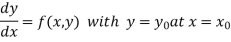
The general first order differential equation
 …. (1)
With the initial condition  … (2)
… (2)
In general, the solution of first order differential equation in one of the two forms:
a) A series for y in terms of power of x, from which the value of y can be obtained by direct solution.
b) A set of tabulated values of x and y.
The case (a) is solved by Taylor’s Series or Picard method whereas case (b) is solved by Euler’s, Runge Kutta Methods etc.
Taylor’s Series Method:
The general first order differential equation
 …. (1)
With the initial condition  … (2)
… (2)
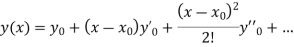
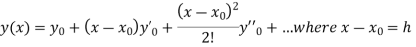
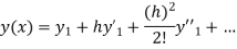
Let  be the exact solution of equation (1), then the Taylor’s series for
  around
  is given by
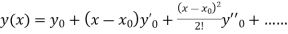 (3)
(3)
If the values of are known, then equation (3) gives apowwer series for y. By total derivatives we have
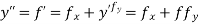 ,
,


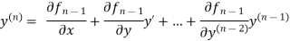
And other higher derivatives of y. The method can easily be extended to simultaneous and higher –order differential equations. In general,
Putting  in these above results, we can obtain the values of
  finally, we substitute these values of
  in equation (2) and obtain the approximate value of y; i.e., the solutions of (1).
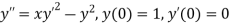
Example1: Solve ,
,  using Taylor’s series method and compute
  .
.
Here 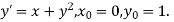 This implies that
 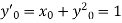 .
.
Differentiating, we get
 .
.
 .
.

 .
.
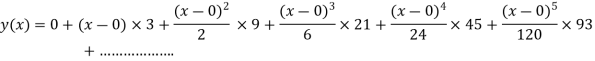
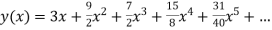
The Taylor’s series at  ,
,


 (1)
(1)
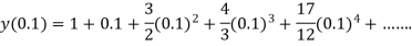
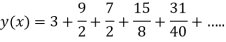
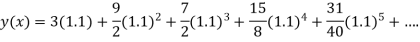
At  in equation (1) we get
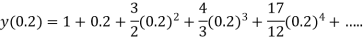
At  in equation (1) we get
Example2: Using Taylor’s series method, find the solution of
At  ?
?
Here 
At  implies that
 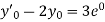 or
or 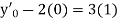 or
or 
Differentiating, we get
 implies that
  or
or  .
.
 implies that
  or
or 
 implies that
  or
or 
 implies that
 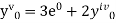 or
or 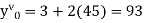
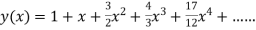
The Taylor’s series at  ,
,
 (1)
(1)
At  in equation (1) we get


At  in equation (1) we get

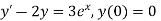
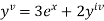
Example3: Solve  numerically, start from
  and carry to
  using Taylor’s series method.
Here  .
.
We have 
Differentiating, we get
 implies that
  or
or 
 implies that
  or
or  .
.
 implies that
 implies that
The Taylor’s series at  ,
,
Or 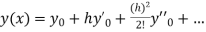


Here 


The Taylor’s series

 .
.
The general first order differential equation
With the initial condition 
4.2.1 Euler’s method:
In this method the solution is in the form of a tabulated values.
Integrating both side of the equation (i) we get
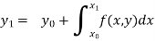
Assuming that  in
in  this gives Euler’s formula
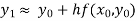
In general formula
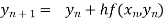 , n=0,1, 2,….
Error estimate for the Euler’s method


Example1: Use Euler’s method to find y (0.4) from the differential equation
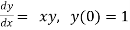 with h=0.1
Given equation 
Here 
We break the interval in four steps.
So that 
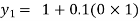
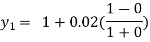
By Euler’s formula
 , n=0,1,2,3 ……(i)
For n=0 in equation (i) we get


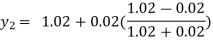
For n=1 in equation (i) we get

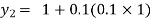
 .01
.01
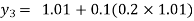
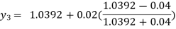
For n=2 in equation (i) we get


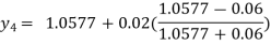
For n=3 in equation (i) we get


Hence y (0.4) =1.061106.
Example2: Using Euler’s method solve the differential equation for y at x=1 in five steps
Given equation 
Here 
No. Of steps n=5 and so that 
So that 
Also 
By Euler’s formula
 , n=0,1,2,3,4 ……(i)
For n=0 in equation (i) we get


For n=1 in equation (i) we get


For n=2 in equation (i) we get


For n=3 in equation (i) we get


For n=4 in equation (i) we get


Hence 
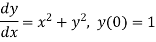
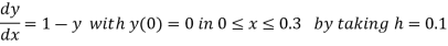
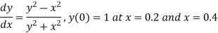
Example3: Given  with the initial condition y=1 at x=0.Find y for x=0.1 by Euler’s method (five steps).
Given equation is 
Here 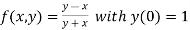
No. Of steps n=5 and so that 
So that 
Also 
By Euler’s formula
 , n=0,1,2,3,4 ……(i)
For n=0 in equation (i) we get


For n=1 in equation (i) we get


For n=2 in equation (i) we get


For n=3 in equation (i) we get


For n=4 in equation (i) we get


Hence 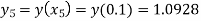
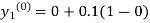
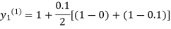
4.2.2 Modified Euler’s Method:
Instead of approximating 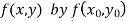 as in Euler’s method. In the modified Euler’s method, we have the iteration formula
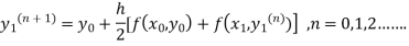
Where  is the nth approximation to
  .The iteration started with the Euler’s formula
Example1: Use modified Euler’s method to compute y for x=0.05. Given that
Result correct to three decimal places.
Given equation 
Here 
Take h =  = 0.05
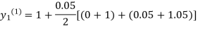
By modified Euler’s formula the initial iteration is

 )
)

The iteration formula by modified Euler’s method is
 -----(i)
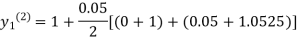
For n=0 in equation (i) we get

Where 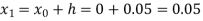 and
and  as above

For n=1 in equation (i) we get


For n=3 in equation (i) we get

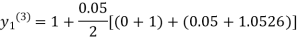

Since third and fourth approximation are equal.
Hence y=1.0526 at x = 0.05 correct to three decimal places.
Example2: Using modified Euler’s method, obtain a solution of the equation
Given equation 
Here 
By modified Euler’s formula the initial iteration is


The iteration formula by modified Euler’s method is
 -----(i)
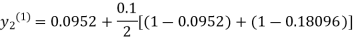
For n=0 in equation (i) we get

Where  and
and  as above

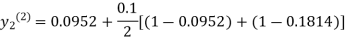
For n=1 in equation (i) we get

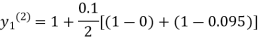

For n=2 in equation (i) we get

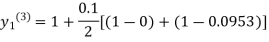

For n=3 in equation (i) we get

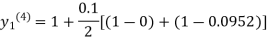

Since third and fourth approximation are equal.
Hence y=0.0952 at x=0.1
To calculate the value of  at x=0.2
By modified Euler’s formula the initial iteration is

The iteration formula by modified Euler’s method is
 -----(ii)
For n=0 in equation (ii) we get

 1814
1814
For n=1 in equation (ii) we get

 1814
1814
Since first and second approximation are equal.
Hence y = 0.1814 at x=0.2
To calculate the value of  at x=0.3
By modified Euler’s formula the initial iteration is

The iteration formula by modified Euler’s method is
 -----(iii)
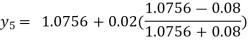
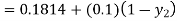
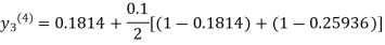
For n=0 in equation (iii) we get

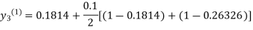
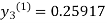
For n=1 in equation (iii) we get

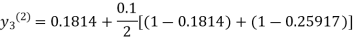
For n=2 in equation (iii) we get


For n=3 in equation (iii) we get

Since third and fourth approximation are same.
Hence y = 0.25936 at x = 0.3
This method is more accurate than Euler’s method.
Consider the differential equation of first order
Let  be the first interval.
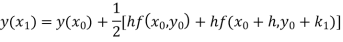
A second order Runge Kutta formula
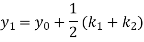
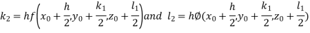
Where 
Rewrite as
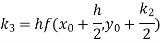
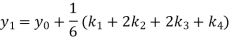
A fourth order Runge Kutta formula:

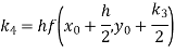
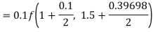
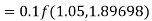
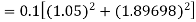
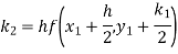
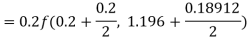
Where 


Example1: Use Runge Kutta method to find y when x=1.2 in step of h=0.1 given that
Given equation 
Here 
Also 
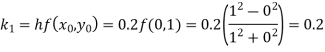
By Runge Kutta formula for first interval


Again 
A fourth order Runge Kutta formula:

To find y at 


A fourth order Runge Kutta formula:


Example2: Apply Runge Kutta fourth order method to find an approximate value of y for x=0.2 in step of 0.1, if
Given equation 
Here 
Also 
By Runge Kutta formula for first interval


A fourth order Runge Kutta formula:


Again 


A fourth order Runge Kutta formula:


Example3: Using Runge Kutta method of fourth order, solve
Given equation 
Here 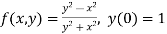
Also 
By Runge Kutta formula for first interval


 )
)


A fourth order Runge Kutta formula:
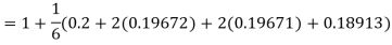

Hence at x = 0.2 then y = 1.196
To find the value of y at x=0.4. In this case 


A fourth order Runge Kutta formula:


Hence at x = 0.4 then y=1.37527
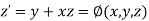
The second order differential equation

Let  then the above equation reduces to first order simultaneous differential equation
Then 
This can be solved as we discuss above by Runge Kutta Method. Here  for
for  and
and  for
for  .
.
A fourth order Runge Kutta formula:

Where 


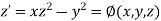
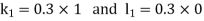
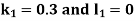
Example1: Using Runge Kutta method of order four, solve  to find
Given second order differential equation is

Let  then above equation reduces to
Or 
 (say)
(say)
Or  .
.
By Runge Kutta Method we have


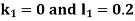


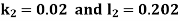
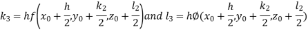


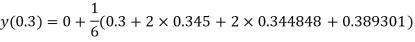
A fourth order Runge Kutta formula:


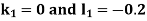
Example2: Using Runge Kutta method, solve
 for
for  correct to four decimal places with initial condition
 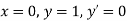 .
.
Given second order differential equation is
Let  then above equation reduces to
Or 
 (say)
(say)
Or 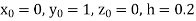 .
.
By Runge Kutta Method we have


A fourth order Runge Kutta formula:


And 
 .
.
Example3: Solve the differential equations
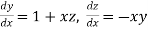 for
for 
Using four order Runge Kutta method with initial conditions 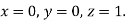
Given differential equation are
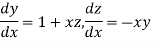
Let 
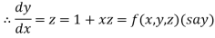
And 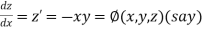
Also 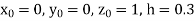
By Runge Kutta Method we have


A fourth order Runge Kutta formula:

And 
 .
.
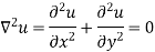
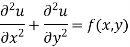
The general linear partial differential equation of the second order in two independent variables is of the form.
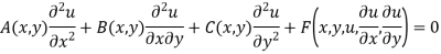
Such a PDE is said to be
- Elliptic: if

- Parabolic: if

- Hyperbolic: if

Example: Classify the equation 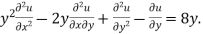
Here 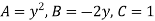
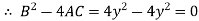
Hence the equation is parabolic.
Finite Difference Approximation
We construct a rectangular region R in the xy- plane and divide into network of sides  and
and  . The intersection points of the dividing lines are called the mesh point, nodal point or grid points.
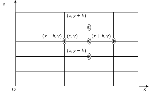
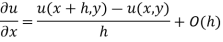
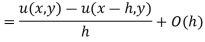
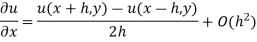
Then the finite difference approximation for the partial derivative in x-direction is
And 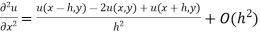
For 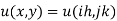 the above approximation is
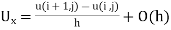 …. (1)
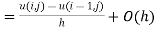 … (2)
… (2)
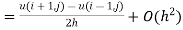 … (3)
… (3)
And 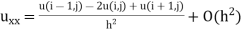 … (4)
… (4)
Similarly, we have the approximations for the derivatives with respect to y
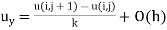 …. (5)
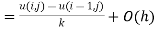 …. (6)
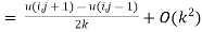 … (7)
… (7)
And 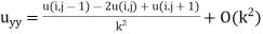 …. (8)
Replacing the derivatives in any partial differential equation by their corresponding difference approximation (1) to (8), we obtain the finite difference similar to the given equations.
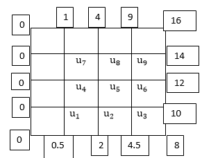
The Laplace’s equation
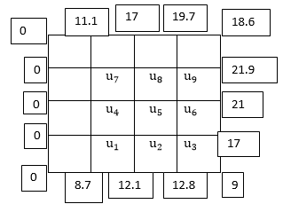
Consider the Laplace’s equation in a region R with boundary C. Let R be a square region so that it can be divided into network of small squares of side h. Let the values of  on the boundary C be given by
  and let the interior mesh points be as in figure
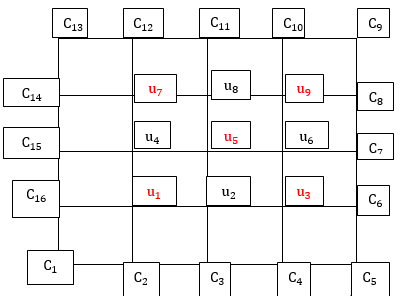
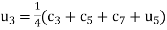
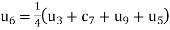
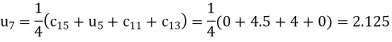
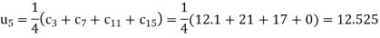
The approximate function values at the interior point of the mesh can be calculated by the diagonal five-point formula of 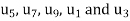 in this order
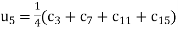 (bigger +)
 (X form)
 (X form)
 (X form)
 (X form)
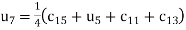
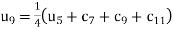
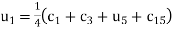
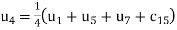
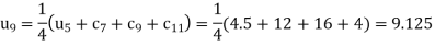
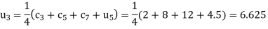
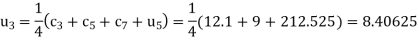
Similarly, the remaining quantities are calculated by using standard five-point diagonal formulas.
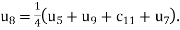 (+ form)
 (+ form)
 (+ form)
 (+ form)
In this way all  are computed.
Example1: Solve the Laplace’s equation  in the domain
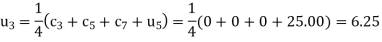
The initial values using five diagonal formula we have
Here  ,
, 
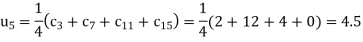

The remaining quantities are calculated by using standard five-point diagonal formulas.


Hence  and
and  .
.
Example2: Solve the Laplace’s equation for
The initial values using five diagonal formula we have
Here  ,
, 


The remaining quantities are calculated by using standard five-point diagonal formulas.


Hence  and
and 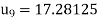 .
.
The Laplace’s equation

And the Poisson’s equation
Are the example of elliptic partial differential equation.
The Poisson’s equation

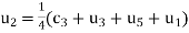
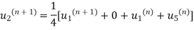
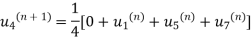
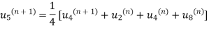
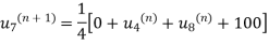
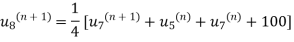
This can be solved by interior mesh points of a square network when the boundary values are known. The standard five-point formula for Poisson’s equation is

After using the above formula, we get the linear equations in the pivotal values 
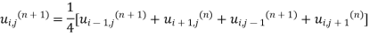
Then these are solved by Gauss Seidel Iteration formula
 .
.
Example1: Solve the elliptical equation for
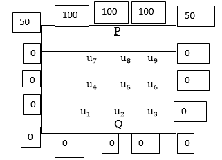
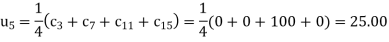
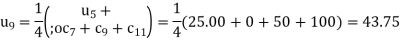
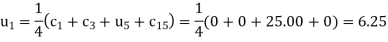
The initial values using five diagonal formula we have
Here  ,
, 

The remaining quantities are calculated by using standard five-point diagonal formulas.


The Above is symmetric about PQ, so that 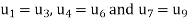 .
.
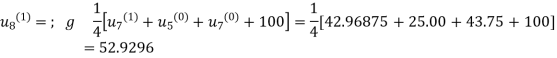
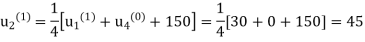
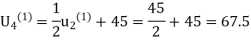
We will have iteration process using the Gauss Seidel Formula
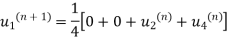
First iteration: Putting  we get


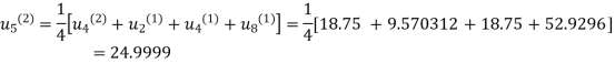
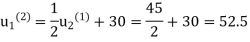
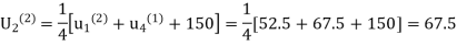
Second Iteration: Putting  , we get


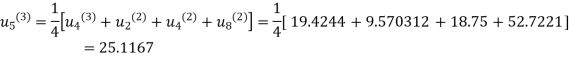
Third Iteration: Putting  , we get


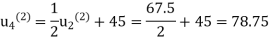
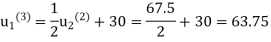
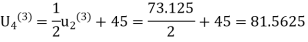
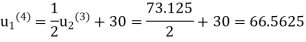
Fourth Iteration: Putting  , we get


Fifth iteration: Putting n=4 we get


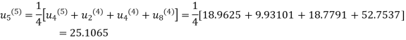

 .
.
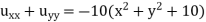
Example2: Solve the Poisson equation
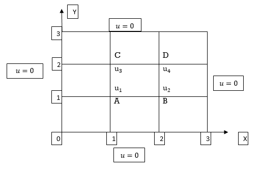
Let the point be defined by  At the point A,
  . The standard five-point formula at point A is

Or 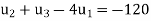
Or 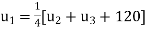 ….(i)
….(i)
Again, the standard five-point formula at the point B is

Or 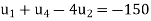
Or 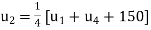 ...(ii)
Similarly, the standard five-point formula at the point C

Or 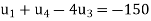
Or 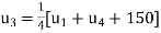 …...(iii)
Similarly, the standard five-point formula at the point D

Or 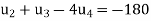
Or 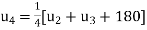 …. (iv)
From (ii) and (iii) we get  =
= . Hence the iteration formula we have
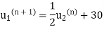
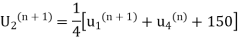
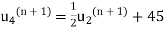 .
.
First iteration: Putting  . Hence, we obtain
Second iteration: Putting n=1, we get
Third iteration: Putting n=2, we get

Fourth iteration: Putting n=3, we get

Fifth iteration: Putting n=4, we get


Sixth iteration: Putting n=5, we get

Since last two iteration are approximately equal, hence
 .
.
The example of parabolic is one dimensional heat conduction equation
 ... (1)
Where  is the diffusivity of the substance.
Consider a rectangular mesh in  plane.
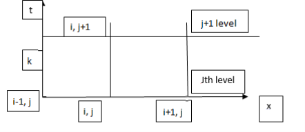
The spacing in x-direction is h and in t direction is k. Let the mesh point  or simply
  we get
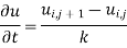
And 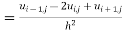
Substituting these in equation (1) we get
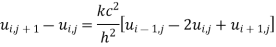
Or  … (2)
… (2)
Where  is the mesh ratio parameter.
This formula gives the value of u at position  mesh points I nterms of known values of
  and
and  at the instant
  . It gives the relation between two-time level therefore known as two level formula.
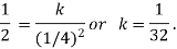
Also named as Schmidt explicit formula and is true for  .
.
At  the above formula reduces to
 ..(3)
..(3)
Is known as Bendre-Schmidt recurrence relation which gives the value of u at internal mesh points with the help of boundary conditions.
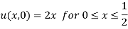
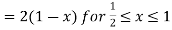
Example1: Solve the equation  with the conditions
  . Assume
 . Tabulate u for
  choosing appropriate value of k?
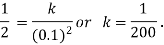
Here 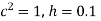 and let
  ,
,
Since 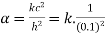
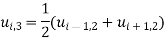
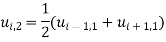
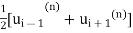
 The Bendre-Schmidt recurrence formula we have
 ….(i)
….(i)
Also given  .
.
 for all values of j, i.e., the entries in the first and the last columns are zero.
Since 
 (Using
For  .
.
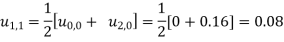
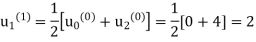
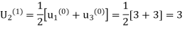
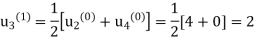
Putting 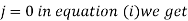
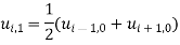
Putting  successively we get
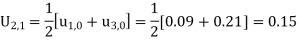
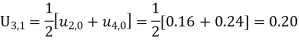
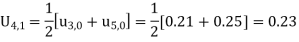
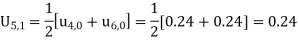
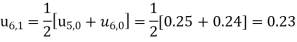
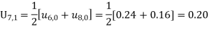
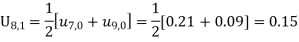
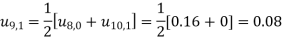
These will give the entries in the second row.
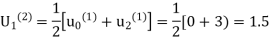
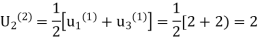
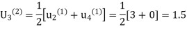
Putting  in equation (i), we will get the entries of the third row.

Similarly,  successively in (i), the entries of the fourth rows are
Obtained.
Hence the values of  are as given in the below the table:
 | 0 | 1 | 2 | 3 | 4 | 5 | 6 | 7 | 8 | 9 | 10 |
0 | 0 | 0.09 | 0.16 | 0.21 | 0.24 | 0.25 | 0.24 | 0.21 | 0.16 | 0.09 | 0 |
1 | 0 | 0.08 | 0.15 | 0.20 | 0.23 | 0.24 | 0.23 | 0.20 | 0.15 | 0.08 | 0 |
2 | 0 | 0.075 | 0.14 | 0.19 | 0.22 | 0.23 | 0.22 | 0.19 | 0.14 | 0.075 | 0 |
3 | 0 | 0.07 | 0.133 | 0.18 | 0.21 | 0.22 | 0.21 | 0.18 | 0.133 | 0.07 | 0 |
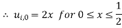
Example2: Solve the heat equation

Subject to the conditions  and
and
 .
.
Take  and k according to Bendre-Schmidt equation.
Here 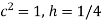 and let
  ,
,
Since 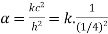
 The Bendre-Schmidt recurrence formula we have
 …. (i)
Also given  .
.
 for all values of j, i.e., the entries in the first and the last columns are zero.
Since 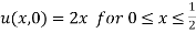
 .
.
 .
.
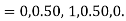
For 
Putting 

Putting  successively we get
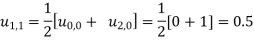
These will give the entries in the second row.
Putting  in equation (i), we will get the entries of the third row.

Similarly,  successively in (i), the entries of the fourth rows are
Obtained.

Hence the values of  are as given in the below the table:
 | 0 | 1 | 2 | 3 | 4 |
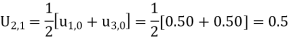
0 | 0 | 0.5 | 1 | 0.5 | 0 |
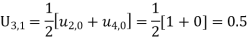
1 | 0 | 0.5 | 0.5 | 0.5 | 0 |
2 | 0 | 0.25 | 0.5 | 0.25 | 0 |
3 | 0 | 0.25 | 0.25 | 0.25 | 0 |
Example3: Use the Bendre-Schmidt formula to solve the heat conduction problem
With the condition 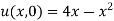 and
and  .
.
Let  we see
  when
when  .
.
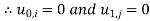
The initial condition are  .
.
Also 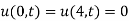 .
.
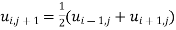
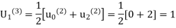
The iteration formula is
 =
=
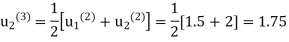
First iteration: Putting n=0, we get
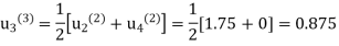
Second iteration: Putting n=1, we get
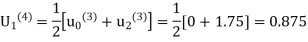
Third Iteration: putting n=3, we get
Fourth Iteration: putting n=3, we get
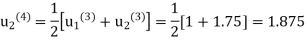
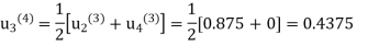
Fifth Iteration: putting n=4, we get
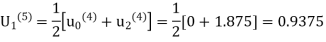
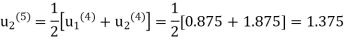
Hence the approximate solution is 
References:
- E. Kreyszig, “Advanced Engineering Mathematics”, John Wiley & Sons, 2006.
- P. G. Hoel, S. C. Port and C. J. Stone, “Introduction to Probability Theory”, Universal Book Stall, 2003.
- S. Ross, “A First Course in Probability”, Pearson Education India, 2002.
- W. Feller, “An Introduction to Probability Theory and Its Applications”, Vol. 1, Wiley, 1968.
- N.P. Bali and M. Goyal, “A Text Book of Engineering Mathematics”, Laxmi Publications, 2010.
- B.S. Grewal, “Higher Engineering Mathematics”, Khanna Publishers, 2000.
- T. Veerarajan, “Engineering Mathematics”, Tata Mcgraw-Hill, New Delhi, 2010
- Higher engineering mathematics, HK Dass
- Higher engineering mathematics, BV Ramana.
- Computer based numerical & statistical techniques, M goyal


