Unit - 3
Numerical Integration
Numerical integration is a process of evaluating or obtaining a definite integral  from a set of numerical values of the integrand f(x).In case of function of single variable, the process is called quadrature.
Trapezoidal rule
Let the interval  be divided into n equal intervals such that
  <
< <…. <
<…. < =b.
=b.
Here .
.
To find the value of .
.
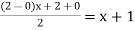
Setting n=1, we get
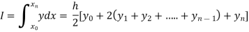
Or I = 
The above is known as Trapezoidal method.
Note: In this method second and higher difference are neglected and so f(x) is a polynomial of degree 1.
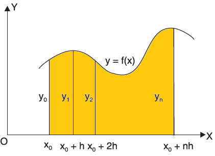
Geometrical Significance: The curve y=f(x), is replaced by n straight lines with the points  (
( );(
);( ) and (
 )……. ;(
 ) and (
 ).
).
The area bounded by the curve y=f(x), the ordinates ,and the x axis is approximately equivalent to the sum of the area of the n trapeziums obtained.
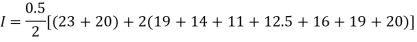
Example1: State the trapezoidal rule for finding an approximate area under the given curve. A curve is given by the points (x, y) given below:

Estimate the area bounded by the curve, the x axis and the extreme ordinates.
We construct the data table:
X | 0 | 0.5 | 1.0 | 1.5 | 2.0 | 2.5 | 3.0 | 3.5 | 4.0 |
Y | 23 | 19 | 14 | 11 | 12.5 | 16 | 19 | 20 | 20 |
Here length of interval h =0.5, initial value a = 0 and final value b = 4
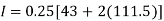
By Trapezoidal method
Area of curve bounded on x axis =

Example2: Compute the value of  ?
?
Using the trapezoidal rule with h=0.5, 0.25 and 0.125.
Here 
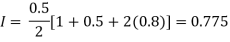
For h=0.5, we construct the data table:
X | 0 | 0.5 | 1 |
Y | 1 | 0.8 | 0.5 |
By Trapezoidal rule

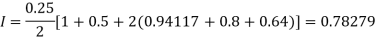
For h=0.25, we construct the data table:
X | 0 | 0.25 | 0.5 | 0.75 | 1 |
Y | 1 | 0.94117 | 0.8 | 0.64 | 0.5 |
By Trapezoidal rule

For h = 0.125, we construct the data table:
X | 0 | 0.125 | 0.25 | 0.375 | 0.5 | 0.625 | 0.75 | 0.875 | 1 |
Y | 1 | 0.98461 | 0.94117 | 0.87671 | 0.8 | 0.71910 | 0.64 | 0.56637 | 0.5 |
By Trapezoidal rule

 [(1+0.5) +2(0.98461+0.94117+0.87671+0.8+0.71910+0.64+0.56637)]

Example3: Evaluate, using trapezoidal rule with five ordinates
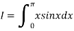
Here 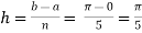
We construct the data table:
X | 0 |  |  |  |  |  |
Y | 0 | 0.3693161 | 1.195328 | 1.7926992 | 1.477265 | 0 |


Key takeaways
- Numerical integration is a process of evaluating or obtaining a definite integral
 from a set of numerical values of the integrand f(x).
Overview-
Generally fundamental theorem of calculus is used find the solution for definite integrals, but sometime integration becomes too hard to evaluate, numerical methods are used to find the approximated value of the integral.
Simpson’s rules are very useful in numerical integration to evaluate such integrals.
Here we will understand the concept of Simpson’s rule and evaluate integrals by using numerical technique of integration.
We find more accurate value of the integration by using Simpson’s rule than other methods
Simpson’s rule
We will study about Simpson’s one-third rule and Simpson’s three-eight rules.
But in order to get these two formulas, we should have to know about the general quadrature formula-
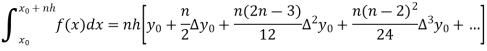
General quadrature formula-
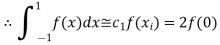
The general quadrature formula is gives as-

Simpson’s one-third and three-eighth formulas are derived by putting n = 2 and n = 3 respectively in general quadrature formula.
Simpson’s one-third and three-eighth formulas are derived by putting n = 2 and n = 3 respectively in general quadrature formula.
Let the interval  be divided into n equal intervals such that
  <
< <…. <
<…. < =b.
=b.
Here .
.
To find the value of .
.
Setting n = 2,

Which is known as Simpson’s 1/3- rule or Simpson’s rule.
Note: In this rule third and higher differences are neglected a so f(x) is a polynomial of degree 2.
Example: Estimate the value of the integral

By Simpson’s rule with 4 strips and 8 strips respectively.
For n=4, we have 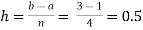
Construct the data table:
X | 1.0 | 1.5 | 2.0 | 2.5 | 3.0 |
Y=1/x | 1 | 0.66666 | 0.5 | 0.4 | 0.33333 |
By Simpson’s Rule


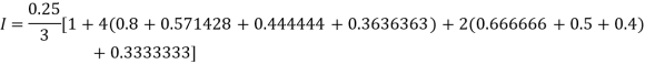
For n = 8, we have 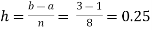
X | 1 | 1.25 | 1.50 | 1.75 | 2.0 | 2.25 | 2.50 | 2.75 | 3.0 |
Y=1/x | 1 | 0.8 | 0.66666 | 0.571428 | 0.5 | 0.444444 | 0.4 | 0.3636363 | 0.333333 |
By Simpson’s Rule


Example: Evaluate 
Using Simpson’s 1/3 rule with  .
.
For  , we construct the data table:
X | 0 |  |  |  |  |  |  |
 | 0 | 0.50874 | 0.707106 | 0.840896 | 0.930604 | 0.98281 | 1 |
By Simpson’s Rule


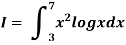
Example: Using Simpson’s 1/3 rule with h = 1, evaluate 
For h = 1, we construct the data table:
X | 3 | 4 | 5 | 6 | 7 |
 | 9.88751 | 22.108709 | 40.23594 | 64.503340 | 95.34959 |
By Simpson’s Rule

= 177.3853
Example: Evaluate the following integral by using Simpson’s 1/3rd rule.

Solution-
First, we will divide the interval into six parts, where width (h) = 1, the value of f(x) is given in the table below-
x | 0 | 1 | 2 | 3 | 4 | 5 | 6 |
f(x) | 1  | 0.5  | 0.2  | 0.1  | 1/17 = 0.05884  | 1/26 = 0.0385  | 1/37 = 0.027  |
Now using Simpson’s 1/3rd rule-

We get-


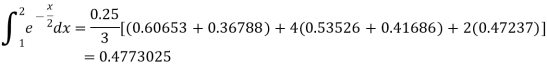
Example: Find the approximated value of the following integral by using Simpson’1/3rd rule.

Solution-
The table of the values-
x | 1 | 1.25 | 1.5 | 1.75 | 2 |
f(x) | 0.60653  | 0.53526  | 0.47237  | 0.41686  | 0.36788  |
Now using Simpson’s 1/3rd rule-

We get-
Example2: Evaluate  Using Simpson’s 1/3 rule with
  .
.
For  , we construct the data table:
X | 0 |  |  |  |  |  |  |
 | 0 | 0.50874 | 0.707106 | 0.840896 | 0.930604 | 0.98281 | 1 |
By Simpson’s Rule


Example3: Using Simpson’s 1/3 rule with h = 1, evaluate
For h = 1, we construct the data table:
X | 3 | 4 | 5 | 6 | 7 |
 | 9.88751 | 22.108709 | 40.23594 | 64.503340 | 95.34959 |
By Simpson’s Rule


= 177.3853
Let the interval  be divided into n equal intervals such that
  <
< <…. <
<…. < =b.
=b.
Here .
.
To find the value of  .
.
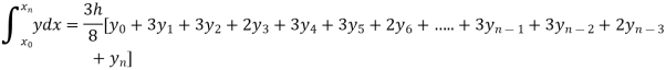
Setting n=3, we get
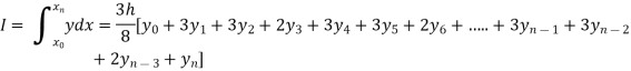
Is known as Simpson’s 3/8 rule which is not as accurate as Simpson’s rule.
Note: In this rule the fourth and higher differences are neglected and so f(x) is a polynomial of degree 3.
Example1: Evaluate 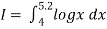
By Simpson’s 3/8 rule.
Let us divide the range of the interval [4, 5.2] into six equal parts.
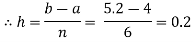
For h=0.2, we construct the data table:
X | 4.0 | 4.2 | 4.4 | 4.6 | 4.8 | 5.0 | 5.2 |
 | 1.3863 | 1.4351 | 1.4816 | 1.5261 | 1.5686 | 1.6094 | 1.6487 |
By Simpson’s 3/8 rule


= 1.8278475
Example2: Evaluate 
Let us divide the range of the interval [0,6] into six equal parts.
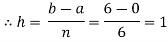
For h=1, we construct the data table:
X | 0 | 1 | 2 | 3 | 4 | 5 | 6 |
 | 1 | 0.5 | 0.2 | 0.1 | 0.0588 | 0.0385 | 0.027 |
By Simpson’s 3/8 rule
 +3(0.0385) +0.027]
=1.3571
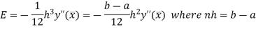
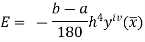
Error in Trapezoidal method
The total error in trapezoidal method is given by
Let  is the largest value of the n quantities on the right hand side of the above equation then
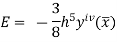
Error in Simpson’s Rule
The error in the Simpson’s rule is given by
Where  is the largest value of the fourth derivative of y(x).
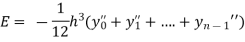
Error in Simpson’s 3/8 Rule
The error in this rule is given by
Where  is the largest value of the derivative of y(x).
Key takeaways
- The general quadrature formula is gives as-
2. Simpson’s one-third rule-

3. Simpson’s three-eighth rule-

Quadrature: It is the process to evaluate the value of the functions at the chosen point, to its exact value for polynomial up to higher degree as possible.
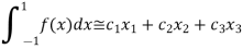
The general form Gaussian quadrature is given by
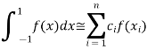
Where  depends on the choice of n (number of points).
Also note that the possible polynomial of degree up to  .
.
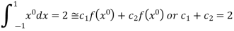
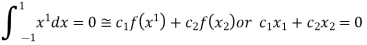
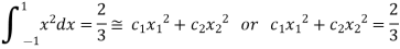
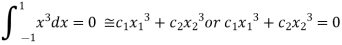
 . …... (1)
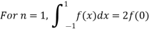
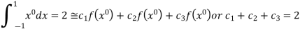
For  point
point
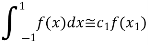
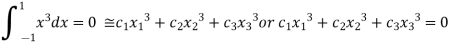
Which gives exact value of the polynomial up to degree 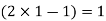 degree
i.e.
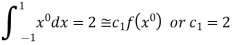
For  point and using (1)
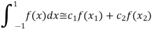
Which gives exact value of the polynomial up to degree  degree
i.e. 
On solving we get
 .
.
Gauss Quadrature 3-point method:
The general form Gaussian quadrature is given by

Where  depends on the choice of n (number of points).
Also note that the possible polynomial of degree up to  .
.
 . …... (1)
For  point
point
Which gives exact value of the polynomial up to degree  degree
i.e. 


On solving we get
 .
.

For n=3, 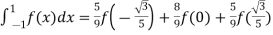
Note: To evaluate 
The above integral can be converted into Gauss quadrature by substituting
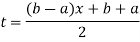


Hence 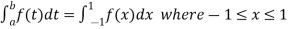 .
.
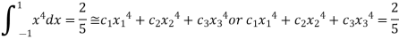
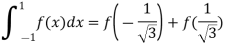
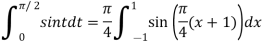
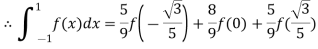
Example: Evaluate 
Here 
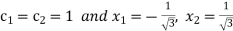
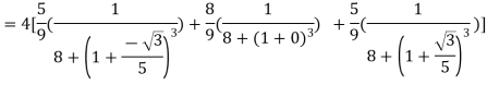
Using  =
=
Also 
For 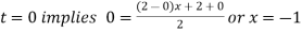
For 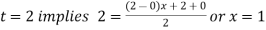
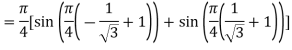
Hence 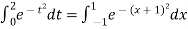
Here 
By Gauss quadrature 3 point rule


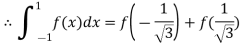
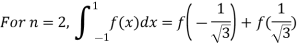
Example: Evaluate  by 2-point Gaussian rule.
Here 
Using  =
=
Also 
For 
For 
Hence 
Here 
By Gauss quadrature 2 point rule
=0.99847
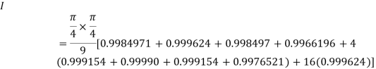
Example: Solve by Gauss quadrature 3-point method 
Given 
Here 
Using 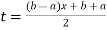 =
=
Also 
For 
For 
Hence 
Here 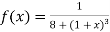
By Gauss quadrature 3 point rule
Hence 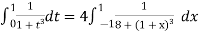

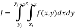
The double integration is defined by

Where .
.
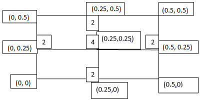
Trapezoidal Rule:
The double integration is defined by

Where .
.
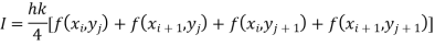
Or
Also, the double integration is defined by

Where .
.

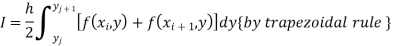
Again, Applying Trapezoidal rule to each term with respect to y.
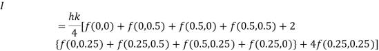
To remember we can use
Example1: Evaluate 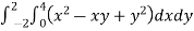
Let 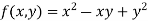
Here the interval of x and y are  and
and  .
.
Let 
Consider the following table:
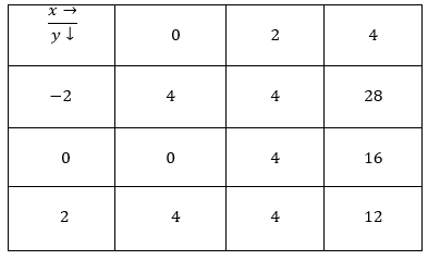
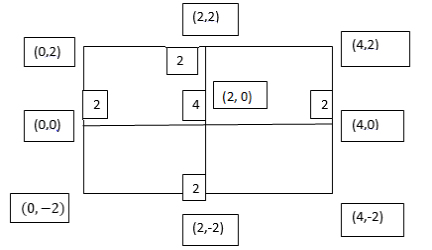
By Trapezoidal Rule

 .
.
Example2: Evaluate 
Let 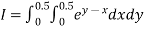
Here 
Let the number of intervals be  .
.
 |
 |
 |
 |
 |

|
 |
 |
 |
 |
 |
 |
 |
 |
 |
 |
By Trapezoidal Rule

 .
.
Example3: Evaluate 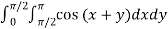
Let 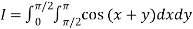
And 
 |
 |
 |
 |
 |
 |
 |
 |
 |
 |
 |
 |
 |
 |
 |
 |
By Trapezoidal Rule


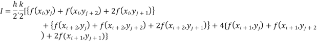
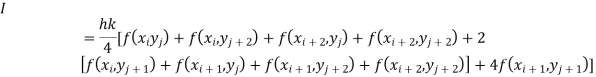
The double integration is defined by
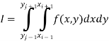
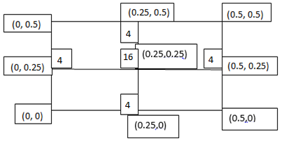
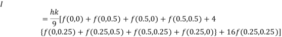
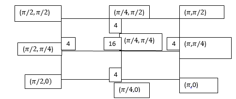
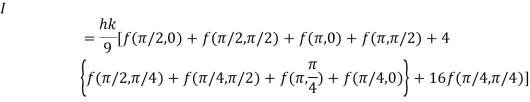
By Simpson’s 1/3 rd Rule
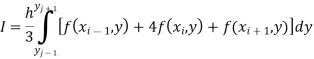
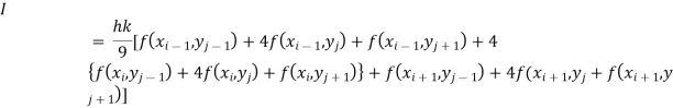

Also, the double integration is defined by
Where .
.
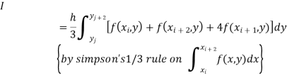
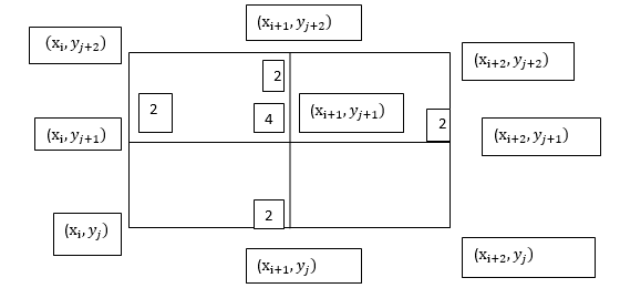
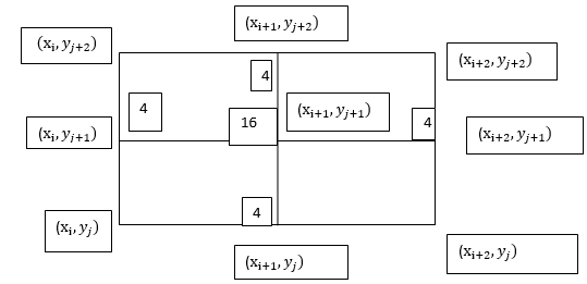
Again, Applying Simpson’s 1/3 rd rule to each term with respect to y.

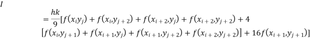
To remember we can use
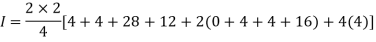
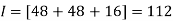
Example1: Evaluate 
Let 
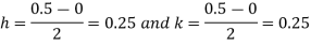
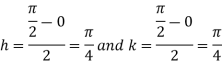
Here the interval of x and y are  and
and  .
.
Let 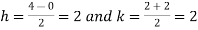
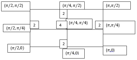
Consider the following table:
 |
 |
 |
 |
 |

|
 |
 |
 |
 |
 |
 |
 |
 |
 |
 |
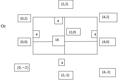
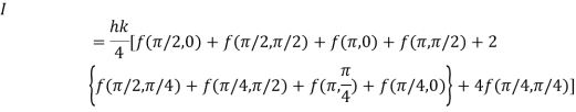
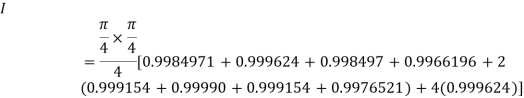
By Simpson’s 1/3 Rule

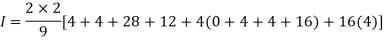
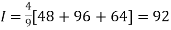 .4444444
Example2: Evaluate 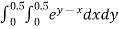
Let 
Here 
Let the number of intervals be  .
.

 |
 |
 |
 |
 |

|
 |
 |
 |
 |
 |
 |
 |
 |
 |
 |
By Simpson’s 1/3 Rule


Example3: Evaluate 
Let 
And 

 |
 |
 |
 |
 |
 |
 |
 |
 |
 |
 |
 |
 |
 |
 |
 |
By Simpson’s 1/3 Rule


References:
- E. Kreyszig, “Advanced Engineering Mathematics”, John Wiley & Sons, 2006.
- P. G. Hoel, S. C. Port and C. J. Stone, “Introduction to Probability Theory”, Universal Book Stall, 2003.
- S. Ross, “A First Course in Probability”, Pearson Education India, 2002.
- W. Feller, “An Introduction to Probability Theory and Its Applications”, Vol. 1, Wiley, 1968.
- N.P. Bali and M. Goyal, “A Text Book of Engineering Mathematics”, Laxmi Publications, 2010.
- B.S. Grewal, “Higher Engineering Mathematics”, Khanna Publishers, 2000.
- T. Veerarajan, “Engineering Mathematics”, Tata Mcgraw-Hill, New Delhi, 2010
- Higher engineering mathematics, HK Dass
- Higher engineering mathematics, BV Ramana.
- Computer based numerical & statistical techniques, M goyal


