Unit - 4

Curve Fitting and Regression Analysis

4.1 Curve Fitting: Least square technique- first order, Power, exponential and quadratic equation

Suppose we are fitting the nth degree curve

To the given values  of two variables x and y.

For that we need to find a, b, c,….,k i.e.  (n+1) constant that would fits best in the above curve of given degree.

Case1:  if m=n+1, we get (n+1) equation by substituting the   unknowns we get a unique solution

Case 2:  if   m>n+1 then no unique solution is possible.  For such cases the method of least square is used.

Let us suppose we get    values corresponding to  respectively. So that, 

……………………………….                         (2)

A curve which has the properties of best fitting curve in  the sense of least square  of given  data,  is called a least square  curve.

Let 

The necessary condition for U to be maximum or minimum are given by

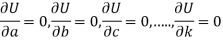
It reduces

………………………………………

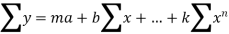
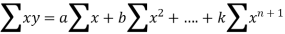
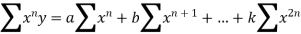
By solving this simultaneous (n+1) equations we get the values of a, b, c,…,k.

The Second order partial derivative of   U is to be calculated and on substitution of a, b, c,…,k we get the minimum value of   U.

Particular:

I)                   When n=1 or  fitting on a straight line:

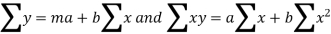
Let the equation be

And its normal equation is

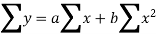
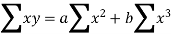
II)                When n=2 or fitting of second degree parabola:

The equation of curve is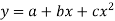 

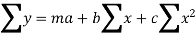
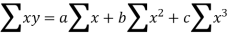
The normal equations are

The values of etc are calculated by means of table (S.D.) and then the value a, b, c…. Are determined.

Example: Fit a straight line to   the following data regarding x as   the independent variables:

The   equation of straight line is

And the normal equations

We construct the data table:

X	Y	XY
0 1 2 3 4	1 1.8 3.3 4.5 6.3	0 1.8 6.6 13.5 25.2	0 1 4 9 16
Total	16.9

Here    (no. Of steps)

Substituting the values from table in normal equations:

16.9=5a+10b

47.1=10a+30b

On solving we getand

Therefore, the required equation of the straight line is .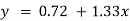

Example: Find the straight line that best fits of the following data by using method of least square.

Sol.

Suppose the straight line

y = a + bx…….. (1)

Fits the best-

Then-

x	y	Xy
1	14	14	1
2	27	54	4
3	40	120	9
4	55	220	16
5	68	340	25
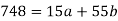
Sum = 15	204	748	55

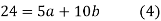
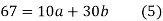
Normal equations are-

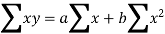
Put the values from the table, we get two normal equations-

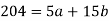
On solving the above equations, we get-

So that the best fit line will be- (on putting the values of a and b in equation (1))

Example2: Fit a second-degree parabola to the following data regarding x as an independent variable:

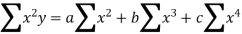
The equation of second-degree curve is

The normal equations are

We construct the data table:

X	Y
0 1 2 3 4	1 5 10 22 38	0 1 4 9 16	0 1 8 27 64	0 1 16 81 256	0 5 20 66 152	0 5 40 198 608
Total	=  76	30	100	354	243	851

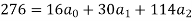
Substituting these   values   from   the table in the above equations

On solving we get and

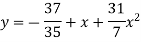
Therefore equation of parabola is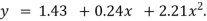

Example: Find the best values of a and b so that y = a + bx fits the data given in the table

Solution.

y = a + bx

x	y	Xy
0	1.0	0	0
1	2.9	2.0	1
2	4.8	9.6	4
3	6.7	20.1	9
4	8.6	13.4	16
x = 10	y ,= 24.0	xy = 67.0

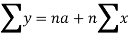
Normal equations, y= na+ bx (2)

On putting the values of

On solving (4) and (5) we get,

On substituting the values of a and b in (1) we get

Example3: Predict y at x = 3.75 by fitting a power curve  to the given data

Given equation is

Taking log on both sides,

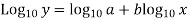
Let    

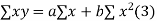
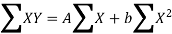
Therefore, its normal equation is

We construct the data table:

				XY
1 2 3 4 5 6	2.98 4.26 5.21 6.10 6.80 7.50	0 0.301030 0.477121 0.602060 0.698970 0.778151	0.474216 0.629410 0.716838 0.785330 0.832509 0.875061	0 0.189471 0.342018 0.472816 0.581899 0.680930	0 0.090619 0.227644 0.362476 0.488559 0.605519
Total

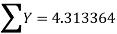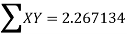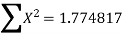Substituting the   values from the   table in the above equations

On solving we get

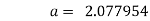
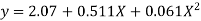
Hence the required equation is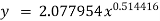

So,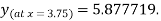 

Example4: Use the   least square   method to determine a and b in the formula

For the following observations

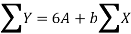
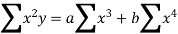
The given equation by

Therefore its rational equation is

We construct the data table:

X	Y
1 2 3 4 5	1.8 5.1 8.9 14.1 19.8	1 4 9 16 25	1 8 27 64 125	1 16 81 264 625	1.8 10.2 26.7 56.4 99.0	1.8 20.4 80.1 225.6 495
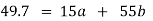
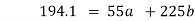
Total	49.7	55	225	987	194.1	822.9

Substituting the above values from the table to the above equations

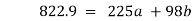
On solving we get

Hence the required equation is 

Example: Fit a second degree parabola to the following data by least squares method.

	1929	1930	1931	1932	1933	1934	1935	1936	1937
	352	356	357	358	360	361	361	360	359

Solution: Taking

Taking 

The equation is transformed to

1929	-4	352	-5	20	16	-80	-64	256
1930	-3	360	-1	3	9	-9	-27	81
1931	-2	357	0	0	4	0	-8	16
1932	-1	358	1	-1	1	1	-1	1
1933	0	360	3	0	0	0	0	0
1934	1	361	4	4	1	4	1	1
1935	2	361	4	8	4	16	8	16
1936	3	360	3	9	9	27	27	81
1937	4	359	2	8	16	32	64	256
Total

Normal equations are

On solving these equations, we get

Example: Find the least squares approximation of second degree for the discrete data

Solution. Let the equation of second degree polynomial be

x	y	Xy
-2	15	-30	4	60	-8	16
-1	1	-1	1	1	-1	1
0	1	0	0	0	0	0
1	3	3	1	3	1	1
2	19	38	4	76	8	16
x=0	y=39	xy=10

Normal equations are

On putting the values of x, y, xy, have

On solving (5), (6), (7), we get,

The required polynomial of second degree is

Example: Fit a second-degree parabola to the following data.

Solution

We shift the origin to (2.5, 0) antique 0.5 as the new unit. This amounts to changing the variable x to X, by the relation X = 2x – 5.

Let the parabola of fit be y = a + bXThe values of X etc. Are calculated as below:

x	X	y	Xy
1.0	-3	1.1	-3.3	9	9.9	-27	81
1.5	-2	1.3	-2.6	4	5.2	-5	16
2.0	-1	1.6	-1.6	1	1.6	-1	1
2.5	0	2.0	0.0	0	0.0	0	0
3.0	1	2.7	2.7	1	2.7	1	1
3.5	2	3.4	6.8	4	13.6	8	16
4.0	3	4.1	12.3	9	36.9	27	81
Total	0	16.2	14.3	28	69.9	0	196

The normal equations are

7a + 28c =16.2; 28b =14.3; 28a +196c=69.9

Solving these as simultaneous equations we get

Replacing X bye 2x – 5 in the above equation we get

Which simplifies to y =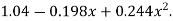

This is the required parabola of the best fit.

4.2 Regression Analysis: Linear regression

I. The simple linear regression is given by

Where 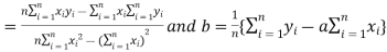, n is number of given data.

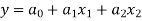
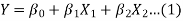
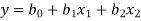
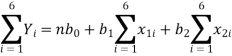
II. The multiple linear regression is

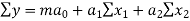
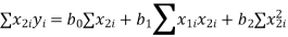
The normal equations are

… (1)

… (2)

… (3)

Example1: Create least   square regression line of set of points

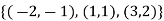
Here is number of data points.

The simple linear regression is given by

Where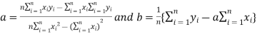

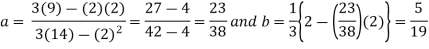
Here which is straight line.

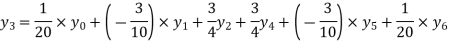
Example2: Find the linear square regression  for the following data.   Also find y when

Here, number of data given. 

The simple linear regression is given by

Where

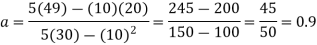
And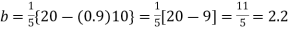

Hence the straight line is given by

Also 

Example3: Fit the equation

To the following data

	0	1	2	3
	10	1	2	3
	12	18	24	30

The multiple linear regression is

The normal equations are

… (1)

… (2)

… (3)

Consider the following table

12	1	10	10	12	120	1	100
18	2	1	2	36	18	4	1
24	3	2	6	72	49	9	4
30	4	3	12	120	90	16	9

Substituting the values from the table in the above equations we get

On solving we get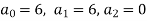

Hence the equation will be

.

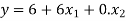Or

4.3 Nonlinear regression & multiple regressions

In multiple regression the number of variables is more than two (with one dependent variable and two or more independent variables).

We know that in agriculture, the crops does not depend on rainfall only but also fertilizers, pesticides, quality of seeds, soil etc.

Thus in multiple regression, the dependent variable Y is a function of more than one independent Variables.

Y= f (X1, X2, X3…, Xk)

Linear multiple regression

Let Y depends on two independent variables X1 and X2,

Then the linear multiple regression problem is to fit the regression plane given by Equation (1) to a

Given set of N triples.

To estimate the coefficient 0, 1, 2, apply the least squares method to minimize

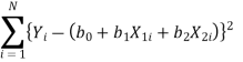
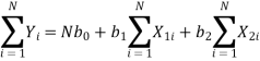
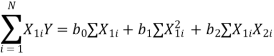
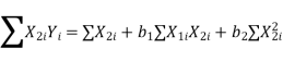
This results in three normal equations given by

Here b0, b1, b2 are the least squares estimates of 0, 1, 2

Example: Fit a regression plane to estimate 0, 1, 2 to the following data of a transport company on the weights of 6 shipments, the distances they were moved and the damage of the goods that was incurred. Estimate the damage when a shipment of 3700 kg is moved to a distance of 260 km.

Sol.

Suppose the dependent variable damage be y, the two independent variables be weight x1 and distance x2. Thus assume the equation of the regression plane as

Where b0, b1, b2 are the estimates of β0, β1, β2.

The three normal equations are

weight (1,000 kg)	distance(100km)	damage
4.0 3.0 1.6 1.2 3.4 4.8	1.5 2.2 1.0 2.0 0.8 1.6	160 112 69 90 123 186	16 9 2.56 1.44 11.56 23.04	2.25 4.84 1.0 4.0 0.64 2.56	6.0 6.0 1.6 2.4 2.72 7.68	640 336 110.4 108 418.2 892.8	240 246.6 69 180 98.4 297.6
18	9.1	740	63.6	15.29	27	250.54	1131.4

The required regression plane we get

For a weight of 3700 kg (x1 = 3.7) and for a distance of 260 km (x2 = 2.6), the damage incurred in rupees is

y (x1 = 3.7, x2 = 2.6) = 14.56+30.109(3.7) +12.16(2.6)

= Rs. 714.5798 ≈ Rs. 715.

4.4 Polynomial regression

Let

Represent a polynomial in X of degree N.

For a given set of N pair of observations (Xi, Yi) the unknowns a0, a1, a2, . . ., aN are estimated by least square method by minimizing

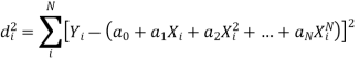
This results in the following (N + 1) normal equations for the determination of (N + 1) unknowns a0, a1, a2, . . ., aN.

Normal equations are

4.5 Lagrange’s   Interpolation

Let , be defined function we get

X				…..
f(x)				……

Where the interval is not necessarily equal. We assume f(x) is a polynomial of degree n.  Then Lagrange’s interpolation formula is given by

Example1: Deduce Lagrange’s formula for interpolation.  The observed values of a function are respectively 168,120,72 and 63 at the four position3,7,9 and 10 of the independent variables. What is the best estimate you can for the value of the function at the position of the independent variable?

We construct the table for the given data:

We need to calculate for x = 6, we need f (6) =?

Here

We get

By Lagrange’s interpolation formula, we have

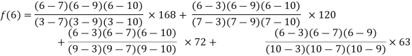
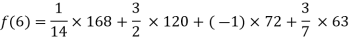
Hence the estimated value for x=6 is 147.

Example2: By means of Lagrange’s formula, prove that

We construct the table:

X	0	1	2	3	4	5	6
Y=f(x)

Here x = 3, f(x)=?

By Lagrange’s formula for   interpolation

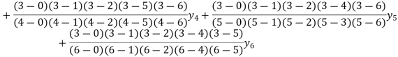
Hence proved.

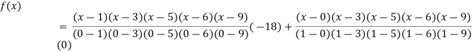
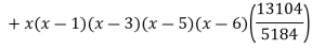
Example3: find the polynomial of fifth degree from the following data

Here

We get 

By Lagrange’s interpolation formula

4.6 Numerical interpolation and differentiation using Newton’s forward method

Interpolation

Definition: Interpolation  is a technique of  estimating the value of  a  function for any  intermediate value of the  independent  variable while  the process  of  computing the  value of the function outside the given range is called   extrapolation.

Let be a function of x.

The table given below gives corresponding values of y for different values of x.

X				….
y= f(x)				….

The process of finding the values of y corresponding to any value of x which lies between   is called interpolation.

If the given function is a polynomial it is polynomial interpolation and given function is known as interpolating polynomial.

Conditions for Interpolation

1)     The function must be   a polynomial of independent variable.

2)     The function   should be either increasing or decreasing function.

3)     The value of   the function should be increase or decrease uniformly.

Finite Difference

Let be a function of x. The table given below gives corresponding values of y for different values of x.

x				….
y= f(x)				….

a)     Forward Difference:  Then  are called differences of y, denoted by 

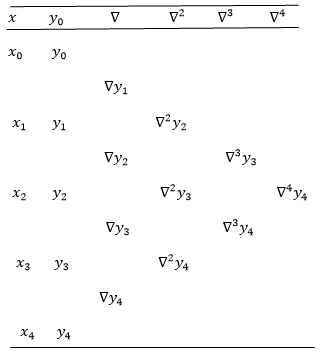
The symbol is called the forward difference operator.  Consider the forward difference table below:

Where

And third forward difference so on.

b)    Backward Difference:

The  difference are called first  backward difference and  is denoted by  Consider the backward  difference  table  below:

		
		         

Where

And third backward differences so on.

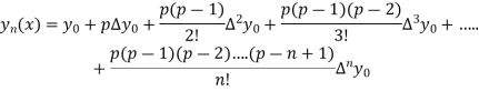
Newton Forward Difference formula:

This method is useful for interpolation near the beginning of a set of tabular values.

Where

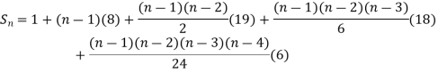
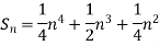
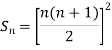
Example1: Using Newton’s forward difference formula, find the sum

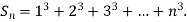
Putting

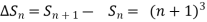
It   follows that

Since is a fourth-degree polynomial in n.

Further,

By Newton Forward Difference Method

Example2:  Given  find   , by using Newton forward interpolation method.

Let 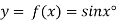 , then

	0.7071	0.7660	-	0.8192	0.8660

The table of forward finite difference is given below:

45           50           55            60	0.7071            0.7660           0.8192            0.8660	0.0589          0.0532          0.0468	-0.0057        -0.0064	-0.0007

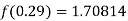
By Newton forward difference method

Here initial value = 45, difference of interval h = 5 and the value to be calculated at x=52.

By Formula

Example3: Find the missing term in the following:

	0	1	2	3	4
	1	3	9	?	81

Let

First we construct the forward difference table:

0       1        2        3        4	1       3       9         81	2         6	4

Now,

Newton Backward Difference Method:

This method is useful for interpolation near the ending of a set of tabular values.

Where 

Example1:  Find from the following table:

	0.20	0.22	0.24	0.26	0.28	0.30
	1.6596	1.6698	1.6804	1.6912	1.7024	1.7139

Consider the backward difference method

0.20         0.22         0.24         0.26         0.28         0.30	1.6596      1.6698      1.6804      1.6912     1.7024       1.7139	0.0102       0.0106      0.0108      0.0112     0.0115	0.0004    0.0002    0.0004    0.0003	-0.0002    0.0002   -0.0001	0.0004   -0.0003	-0.0007

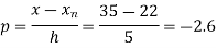
Here

By Newton backward difference formula

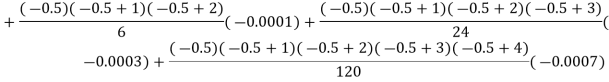
Example2: The following table give the amount of a chemical dissolved in water:

Temp.
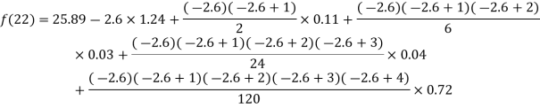
Solubility	19.97	21.51	22.47	23.52	24.65	25.89

Compute the amount dissolve at

Consider the following backward difference table:

Temp.  x	Solubility y
10     15     20     25     30     35	19.97      21.51     22.47     23.52      24.65      25.89	1.54     0.96    1.05     1.13     1.24	-0.58      0.09      0.08      0.11	0.67     -0.01      0.03	-0.68     0.04	0.72

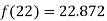
Here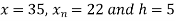

By Newton Backward difference formula

Example3: The following are the marks obtained by 492 candidates in a certain examination

Find out the number of candidates:

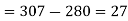
a)     Who secured more than 48 but not more than 50 marks?

b)    Who secured less than 48 but not less than 45 marks?

Consider the forward difference table given below:

Marks  upto x	No. Of candidates y
40       45       50       55       60       65	210   210+43=253   253+54=307   307+74=381   381+32=413   413+79= 492	43       54       74       32        79	11     20     -42      47	9     -62      89	-71        151	222

Here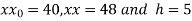 

By Newton Forward Difference formula

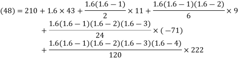
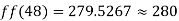
a)     No. Of  candidate secured more than 48  but  not more than  50 marks

b)    No. Of  candidate secured less than 48 but  not  less  than 45 marks

4.7 Inverse Interpolation (Lagrange’s Method only)

Given a set of values of x and y, the process of finding the value of x for a certain value of y is called inverse interpolation.

Lagrange’s Inverse interpolation:

Let , be defined function we get

x				…..
f(Y)				……

Where the interval is not necessarily equal. We assume f(x) is a polynomial of degree n.  Then Lagrange’s inverse interpolation formula is given by

Example1: Use the inverse interpolation to find value of x at for the following data:

Here , we have the data

The Lagrange’s inverse interpolation formula is given by

.

Example2: Use the inverse   Lagrange’s method to find the root of the equation , give data

Here , we have the data

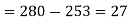
Also.

The Lagrange’s inverse interpolation formula is given by

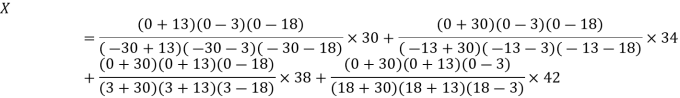
Thus, the approximate   root of the given equation is .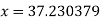

Example3: Find the value of x at for the following data:

Here , we have the data

Also.

The Lagrange’s inverse interpolation formula is given by

Thus the value

References:

1. E. Kreyszig, “Advanced Engineering Mathematics”, John Wiley & Sons, 2006.
2. P. G. Hoel, S. C. Port and C. J. Stone, “Introduction to Probability Theory”, Universal Book Stall, 2003.
3. S. Ross, “A First Course in Probability”, Pearson Education India, 2002.
4. W. Feller, “An Introduction to Probability Theory and Its Applications”, Vol. 1, Wiley, 1968.
5. N.P. Bali and M. Goyal, “A Text Book of Engineering Mathematics”, Laxmi Publications, 2010.
6. B.S. Grewal, “Higher Engineering Mathematics”, Khanna Publishers, 2000.
7. T. Veerarajan, “Engineering Mathematics”, Tata McGraw-Hill, New Delhi, 2010
8. Higher engineering mathematics, HK Dass
9. Higher engineering mathematics, BV Ramana.
10. Computer based numerical & statistical techniques, M goyal