Unit - 5
Statistics
Professor Bowley defines the average as-
“Statistical constants which enable us to comprehend in a single effort the significance of the whole”
An average is a single value that is the best representative for a given data set.
Measures of central tendency show the tendency of some central values around which data tend to cluster.
The following are the various measures of central tendency-
1. Arithmetic mean
2. Median
3. Mode
4. Weighted mean
5. Geometric mean
6. Harmonic mean
The arithmetic mean or mean-
The arithmetic mean is a value which is the sum of all observation divided by a total number of observations of the given data set.
If there are n numbers in a dataset-  then the arithmetic mean will be-

If the numbers along with frequencies are given then mean can be defined as-

This is known as direct method.
Example 1: Find the mean of 20, 22, 25, 28, 30.
Solution:

Example-2: Find the mean of 26, 15, 29, 36, 35, 30, 14, 21, 25.
Sol.


Example 3: Find the mean of the following:
Numbers | 8 | 10 | 15 | 20 |
Frequency | 5 | 8 | 8 | 4 |
Solution:


Example-4: Find the mean of the following dataset.
X | 20 | 30 | 40 |
F | 5 | 6 | 4 |
Sol.
We have the following table-
X | F | Fx |
20 | 5 | 100 |
30 | 6 | 180 |
40 | 7 | 160 |
| Sum = 15 | Sum = 440 |
Then Mean will be-


(b) Shortcut method
Let be the assumed mean, d the deviation of the variate
  from
from . Then


Example 5: Find the arithmetic mean for the following distribution:
Class | 0-10 | 10-20 | 20-30 | 30-40 | 40-50 |
Frequency | 7 | 8 | 20 | 10 | 5 |
Solution:
Let assumed mean 
Class | Mid-value  | Frequency  |  |  |
0-10 10-20 20-30 30-40 40-50 | 5 15 25 35 45 | 7 8 20 10 5 | -20 -10 0 10 5 | -140 -80 0 100 100 |
Total |
|
| 50 | -20 |

(c) Step deviation method
Let be the assumed mean,
  the width of the class interval and

Example 6. Find the arithmetic mean of the data given in example by step deviation method
Solution. Let 
Class | Mid‐value  | Frequency  |  |  |
     |      |      |      |      |
Total |
|  |
|  |

Median is the mid-value of the given data when it is arranged in ascending or descending order.
1. If the total number of values in the data set is odd then the median is the value of  item.
item.
Note-The data should be arranged in ascending r descending order
2. If the total number of values in the data set is even then the median is the mean of the  item.
item.
Example:
Find the median of 
Solution:
Total number of items =7
The middle item
Median=Value of the 4th item=10
Example: Find the median of the data given below-
7, 8, 9, 3, 4, 10
Sol.
Arrange the data in ascending order-
3, 4, 7, 8, 9, 10
So there total 6 (even) observations, then-


Median for grouped data-

Here,


Example:
Find the value of Median from the following data.
No. Of days for which absent (Less than) | 5 | 10 | 15 | 20 | 25 | 30 | 35 | 40 | 45 |
No. Of students | 29 | 224 | 465 | 582 | 634 | 644 | 650 | 653 | 655 |
Solution: The given cumulative frequency distribution will first be converted into ordinary frequency as under
Class Interval | Cumulative frequency | Ordinary frequency |
0-5 5-10  15-20 20-25 25-35 30-35 35-40 40-45 | 29  465 582 634 644 650 653 655 | 29=29 224-29=195 465-224=  582-465=117 634-582=52 644-634=10 650-644=6 653-650=3 655-653=2 |
Median= size of or 327.5th item
327.5th item lies in 10-15 which is the median class.

Where  stands for lower limit of median class,
N stands for the total frequency,
C stands for the cumulative frequency just preceding the median class,
 stands for class interval
 stands for frequency for the median class.
Median

Example: Find the median of the following dataset-
Class interval | 0-10 | 10-20 | 20-30 | 30-40 | 40-50 |
Frequency | 3 | 5 | 7 | 9 | 4 |
Sol.
Class interval | Frequency | Cumulative frequency |
0 – 10 | 3 | 3 |
10 – 20 | 5 | 8 |
20 – 30 | 7 | 15 |
30 – 40 | 9 | 24 |
40 – 50 | 4 | 28 |

So that median class is 20-30.
Now putting the values in the formula-


So that the median is 28.57
Mode is defined to be the size of the variable which occurs most frequently.
Example:
Find the mode of the following items:
0, 1, 6, 7, 2, 3, 7, 6, 6, 2, 6, 0, 5, 6, 0.
Solution:
6 occurs 5 times and no other item occurs 5 or more than 5 times, hence the mode is 6.
Mode for grouped data-

Here,


Emperical formula
Mean – Mode = 3 [Mean – Median]
Example:
Find the mode from the following data:
Age | 0-6 | 6-12 | 12-18 | 18-24 | 24-30 | 30-36 | 36-42 |
Frequency | 6 | 11 | 25 | 35 | 18 | 12 | 6 |
Solution:
Age | Frequency | Cumulative frequency |
0-6 6-12 12-18  24-30 30-36 36-42 | 6 11 25  35   12 6 | 6 17 42 77 95 107 113 |
Mode


Example: Find the mode of the following dataset-
Class interval | 0-10 | 10-20 | 20-30 | 30-40 | 40-50 |
Frequency | 3 | 5 | 7 | 9 | 4 |
Sol.
Class interval | Frequency |
0 - 10 | 3 |
10 – 20 | 5 |
20 – 30 | 7 |
30 – 40 | 9 |
40 – 50 | 4 |
Here the highest frequency is 9. So that the modal class is 40-50,
Put the values in the given data-


Hence the mode is 42.86
According to Spiegel-
“The degree to which numerical data tend to spread about an average value is called the variation or dispersion of data”
The different measures of dispersion are-
1. Range
2. Quartile deviation
3. Mean deviation
4. Standard deviation
5. Variance
Standard deviation:
It is defined as the positive square root of the arithmetic mean of the square of the deviation of the given values from their arithmetic mean. It is denoted by the symbol  .
.

Where  is A.M of the distribution
  . We have more formulae to calculate the standard deviation.


 ….
…. 
In frequency distribution from, we put  where H is generally taken as width of class interval


Shortcut formula to calculate standard deviation-

The square of the standard deviation is called known as a variance.

Example-1: Compute the variance and standard deviation.
Class | Frequency |
0-10 | 3 |
10-20 | 5 |
20-30 | 7 |
30-40 | 9 |
40-50 | 4 |
Sol.
Class | Mid-value (x) | Frequency (f) |  |
0-10 | 5 | 3 | 1470.924 |
10-20 | 15 | 5 | 737.250 |
20-30 | 25 | 7 | 32.1441 |
30-40 | 35 | 9 | 555.606 |
40-50 | 45 | 4 | 1275.504 |
Sum |
|  | 4071.428 |

Then standard deviation,

Example-2: Calculate the standard deviation of the following frequency distribution-
Weight | 60 – 62 | 63 – 65 | 66 – 68 | 69 – 71 | 72 – 74 |
Item | 5 | 18 | 42 | 27 | 8 |
Sol.
Weight | Item (f) | X | d = x – 67 | f.d |  |
60 – 62 | 5 | 61 | -6 | -30 | 180 |
63 – 65 | 18 | 64 | -3 | -54 | 162 |
66 – 68 | 42 | 67 | 0 | 0 | 0 |
69 – 71 | 27 | 70 | 3 | 81 | 243 |
72 – 74 | 8 | 73 | 6 | 48 | 288 |
Total |
100 |
|
|
45 |
873 |


Example: Calculate S.D for the following distribution.
Wages in rupees earned per day | 0-10 | 10-20 | 20-30 | 30-40 | 40-50 | 50-60 |
No. Of Labourers | 5 | 9 | 15 | 12 | 10 | 3 |
Solution:
Wages earned C.I | Mid value  | Frequency |  |  |  |
52 | 5 | 5 | -2 | -10 | 20 |
153 | 15 | 9 | -1 | -9 | 9 |
25 | 25 | 15 | 0 | 0 | 0 |
35 | 35 | 12 | 1 | 12 | 12 |
45 | 45 | 10 | 2 | 20 | 40 |
55 | 55 | 3 | 3 | 9 | 27 |
Total | - |  |  |  |  |
Using formula,


Coefficient of variation
Coefficient of variation can be calculated as-

Note- The lower value of C.V, the more constancy of data
Example- If student A has a mean 50 with SD 10.Another student B has a mean of 30 with SD = 3.
Which one is the best performer?
Sol. We calculate C.V.-


And

Here B has a lower C.V. So that student B is the best performer.
Example: Calculate coefficient variation for the following frequency distribution.
Wages in Rupees earned per day | 0-10 | 10-20 | 20-30 | 30-40 | 40-50 | 50-60 |
No. Of Labourers | 5 | 9 | 15 | 12 | 10 | 3 |
Solution:
We already calculated

Now,
A.M 

A.M 
 Coefficient of Variation


Standard Error (S.E.) is the standard deviation of the sampling distribution of a statistic S. It gives an index of the precision of the estimate of the parameters. As the sample size n increases, S.E. Decreases. Standard error plays an important role in large sample theory and forms the basis in tests of hypothesis.
The standard error (SE) of a statistic is the approximate standard deviation of a statistical sample population. The standard error is a statistical term that measures the accuracy with which a sample distribution represents a population by using standard deviation.
The relationship between the standard error and the standard deviation is such that, for a given sample size, the standard error equals the standard deviation divided by the square root of the sample size.
Standard deviation and standard error of the mean are both statistical measures of variability. While the standard deviation of a sample depicts the spread of observations within the given sample regardless of the population mean, the standard error of the mean measures the degree of dispersion of sample means around the population mean.
The standard error is calculated as

 is the standard deviation and n is the sample size.
This is one of the simplest measures of dispersion. The difference between the maximum and minimum value of the dataset is known as the range.
Range = Max. Value – Min. Value
Example- Find the range of the data- 8, 5, 6, 4, 7, 10, 12, 15, 25, 30
Sol. Here the maximum value is 30 and the minimum value is 4 so that the range is-
30 – 4 = 26
Coefficient of range-
The coefficient of range can be calculated as follows-
Coefficient of Range = 
Quartile deviation-


Example- Find the quartile deviation of the following data-
Class interval | 0-10 | 10-20 | 20-30 | 30-40 | 40-50 |
Frequency | 3 | 5 | 7 | 9 | 4 |
Sol.
Here N/4 = 28/4 = 7 so that the 7’th observation falls in class 10 – 20.
And
3N/4 = 21, and 21’st observation falls in the interval 30 – 40 which is the third quartile.
The quartiles can be calculated as below-

And

Hence the quartile deviation is-

Mean deviation-
The mean deviation can be defined as-

Here A is assumed mean.


Example: Find the mean deviation from the mean of the following data-
Class interval | 0-6 | 6-12 | 12-18 | 18-24 | 24-30 |
Frequency | 8 | 10 | 12 | 9 | 5 |
Sol.
Class interval | Mid-value | Frequency | d = x – a | f.d | |x - 14| | f |x - 14| |
0-6 | 3 | 8 | -12 | -96 | 11 | 88 |
6-12 | 9 | 10 | -6 | -60 | 5 | 50 |
12-18 | 15 | 12 | 0 | 0 | 1 | 12 |
18-24 | 21 | 9 | 6 | 54 | 7 | 63 |
24-30 | 27 | 5 | 12 | 60 | 13 | 65 |
Total |
| 44 |
| -42 |
| 278 |

Then mean deviation from mean-

SKEWNESS:
Skewness denotes the opposite of symmetry. It is lack of symmetry. In a symmetrical series, the mode, the median, and the arithmetic average are identical.
Coefficient of skewness 
KURTOSIS: It measures the degree of peakedness of a distribution and is given by Measure of kurtosis.


Negative skewness Positive skewness A: Mesokurtic B: Leptokurtic
C: Playkurtic

If  , the curve is normal or mesokurtic.
If  , the curve is peaked or leptokurtic.
If  , the curve is flat topped or platykurtic
Example
The first four moments about the working mean 28.5 of a distribution 0.294, 7.144, 42.409 and 454.98. Calculate the moments about the mean. Also evaluate  and comment upon the skewness and kurtosis of the distribution.
Solution:
The first four moments about the arbitrary origin 28.5 are  and
and  .
.
 or
or


Now 

 which indicates considerable skewness of the distribution.
 which shows that the distribution is leptokurtic.
Example
Calculate the median, quartiles and the quartile coefficient of skewness from the following data:
Weight (lbs) | 70-80 | 80-90 | 90-100 | 100-110 | 110-120 | 120-130 | 130-140 | 140-150 |
No. Of Persons | 12 | 18 | 35 | 42 | 50 | 45 | 20 | 8 |
Solution
Here total frequency  =230.
=230.
The cumulative frequency table is
Weight (lbs) | 70-80 | 80-90 | 90-100 | 100-110 | 110-120 | 120-130 | 130-140 | 140-150 |
 | 12 | 18 | 35 | 42 | 50 | 45 | 20 | 8 |
 | 12 | 30 | 65 | 107 | 157 | 202 | 222 | 230 |
Now item which lies in 110-120 group.
 Median or

Also  i.e.
i.e.  is
is  or
or  item which lies in 90-100 group.

Similarly,  i.e.,
i.e., is
is  item which lies in 120-130 group.

Hence quartile coefficient of skewness 
 (approx)
Scatter diagram
A scatter plot is a chart type that is normally used to observe and visually display the relationship between variables. It is also known as a scattergram, scatter graph, or scatter chart.
The data points or dots, which appear on a scatter plot, represent the individual values of each of the data points and also allow pattern identification when looking at the data holistically.
The most common use of the scatter plot is to display the relationship between two variables and observe the nature of such a relationship. The relationships observed can either be positive or negative, non-linear or linear, and/or, strong or weak.
When we plot the corresponding values of two variables, taking one on x-axis and the other
Along y-axis, it shows a collection of dots.

This collection of dots is called a dot diagram or a scatter diagram
Histogram-
Histograms are used to represent the frequency distribution. The histogram looks like bar graph but it groups members into ranges.
In other words- A histogram is the graphical representation of data where data is grouped into continuous number ranges and each range corresponds to a vertical bar.
Histogram consists of a set of rectangles having their heights proportional to the class frequencies, for equal class-intervals. For unequal class-interval, the areas of rectangles are proportional to the frequencies.
Frequency histogram- A Frequency Histogram is a special graph that uses vertical columns to show frequencies
Each bar typically covers a range of numeric values called a bin or class; a bar’s height indicates the frequency of data points with a value within the corresponding bin.
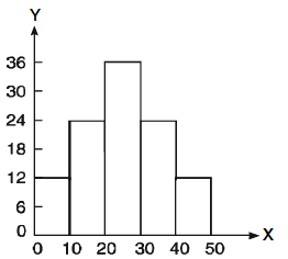
Example: Plot the histogram of the following data
Age | 0-10 | 10-20 | 20-30 | 30-40 | 40-50 |
Persons | 12 | 23 | 35 | 20 | 10 |
Sol.
By taking class intervals on x axis and persons on y axis.
We draw the histogram as below
Pie chart
A pie chart is a type of graph that represents the data in the circular graph. The slices of pie show the relative size of the data. It is a type of pictorial representation of data.
A pie chart requires a list of categorical variables and the numerical variables.
Pie chart is also known as circle chart. A pie chart shows how a total amount is divided between levels of a categorical variable as a circle divided into radial slices.
Pie chart formula =
When two variables are related in such a way that a change in the value of one variable affects the value of the other variable, then these two variables are said to be correlated and there is a correlation between two variables.
Example- Height and weight of the persons of a group.
The correlation is said to be a perfect correlation if two variables vary in such a way that their ratio is constant always.
Basically correlation is the measurement of the strength of a linear relationship between two variables.
In other words, we define the correlation as- if the change in one variable affects a change in other variable, then these two variables are said to be correlated.
For example:
- The correlation between a person’s income and expenditures.
- As the temperature goes up, the demand of ice cream also goes up.
Types of correlation
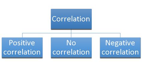
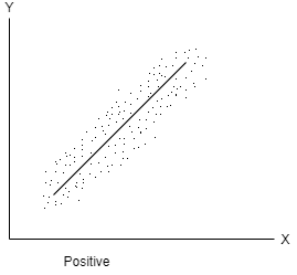
Positive correlation- When both variables move in the same direction, or if the increase in one variable results in a corresponding increase in the other one is called positive correlation.
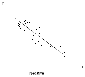
Negative correlation- When one variable increases and other decreases or vice-versa, then the variables said to be negatively correlated.
No correlation- When two variables are independent and do not affect each other then there will be no correlation between the two and said to be un-correlated.
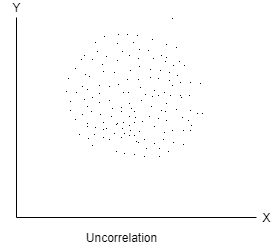
Note- (Perfect correlation)- When a variable changes constantly with the other variable, then these two variables are said to be perfectly correlated.
Scatter plots or dot diagrams
Scatter or dot diagram is used to check the correlation between the two variables.
It is the simplest method to represent a bivariate data.
When the dots in diagram are very close to each other, then we can say that there is a fairly good correlation.
If the dots are scattered then we get a poor correlation.
Karl Pearson’s coefficient of correlation-

Here-  and
and 

Note-
1. Correlation coefficient always lies between -1 and +1.
2. Correlation coefficient is independent of the change of origin and scale.
3. If the two variables are independent then the correlation coefficient between them is zero.
Correlation coefficient | Type of correlation |
+1 | Perfect positive correlation |
-1 | Perfect negative correlation |
0.25 | Weak positive correlation |
0.75 | Strong positive correlation |
-0.25 | Weak negative correlation |
-0.75 | Strong negative correlation |
0 | No correlation |
Example: Find the correlation coefficient between age and weight of the following data-
Age | 30 | 44 | 45 | 43 | 34 | 44 |
Weight | 56 | 55 | 60 | 64 | 62 | 63 |
Sol.
x | y |  |  |  |  | (   |
30 | 56 | -10 | 100 | -4 | 16 | 40 |
44 | 55 | 4 | 16 | -5 | 25 | -20 |
45 | 60 | 5 | 25 | 0 | 0 | 0 |
43 | 64 | 3 | 9 | 4 | 16 | 12 |
34 | 62 | -6 | 36 | 2 | 4 | -12 |
44 | 63 | 4 | 16 | 3 | 9 | 12 |
Sum= 240 |
360 |
0 |
202 |
0 |
70
|
32 |
Karl Pearson’s coefficient of correlation-

Here the correlation coefficient is 0.27.which is the positive correlation (weak positive correlation), this indicates that as age increases, the weight also increases.
Short-cut method to calculate correlation coefficient-

Here,


Example: Find the correlation coefficient between the values X and Y of the dataset given below by using the short-cut method-
X | 10 | 20 | 30 | 40 | 50 |
Y | 90 | 85 | 80 | 60 | 45 |
Sol.
X | Y |  |  |  |  |  |
10 | 90 | -20 | 400 | 20 | 400 | -400 |
20 | 85 | -10 | 100 | 15 | 225 | -150 |
30 | 80 | 0 | 0 | 10 | 100 | 0 |
40 | 60 | 10 | 100 | -10 | 100 | -100 |
50 | 45 | 20 | 400 | -25 | 625 | -500 |
Sum = 150 |
360 |
0 |
1000 |
10 |
1450 |
-1150 |
Short-cut method to calculate correlation coefficient-


A group of n individuals may be arranged in order to merit with respect to some characteristics. The same group would give different orders for different characteristics. Considering the orders corresponding to two characteristics A and B, the correction between these n pairs of rank is called the rank correlation in the characteristics A and B for that group of individuals.
Let  be the ranks of the ith individuals in A and B respectively. Assuming that no two individuals are bracketed equal in either case, each of the variables taking the values 1,2, 3…, n we have

If X, Y be the deviations of x, y from their means, then


Now let, 


Hence the correlation coefficient between these variables is

This is called the rank correlation coefficient and is denoted by 
Example. Ten participants in a contest are ranked by two judges as follows:
x | 1 | 6 | 5 | 10 | 3 | 2 | 4 | 9 | 7 | 8 |
y | 6 | 4 | 9 | 8 | 1 | 2 | 3 | 10 | 5 | 7 |
Calculate the rank correlation coefficient 
Solution. If 

Hence, 
Example. Three judges A, B, C give the following ranks. Find which pair of judges has common approach
A | 1 | 6 | 5 | 10 | 3 | 2 | 4 | 9 | 7 | 8 |
B | 3 | 5 | 8 | 4 | 7 | 10 | 2 | 1 | 6 | 9 |
C | 6 | 4 | 9 | 8 | 1 | 2 | 3 | 10 | 5 | 7 |
Solution. Here n = 10
A (=x) | Ranks by B(=y) | C (=z) |  x-y |  y - z |  z-x | 
|  |  |
1 | 3 | 6 | -2 | -3 | 5 | 4 | 9 | 25 |
6 | 5 | 4 | 1 | 1 | -2 | 1 | 1 | 4 |
5 | 8 | 9 | -3 | -1 | 4 | 9 | 1 | 16 |
10 | 4 | 8 | 6 | -4 | -2 | 36 | 16 | 4 |
3 | 7 | 1 | -4 | 6 | -2 | 16 | 36 | 4 |
2 | 10 | 2 | -8 | 8 | 0 | 64 | 64 | 0 |
4 | 2 | 3 | 2 | -1 | -1 | 4 | 1 | 1 |
9 | 1 | 10 | 8 | -9 | 1 | 64 | 81 | 1 |
7 | 6 | 5 | 1 | 1 | -2 | 1 | 1 | 4 |
8 | 9 | 7 | -1 | 2 | -1 | 1 | 4 | 1 |
Total |
|
| 0 | 0 | 0 | 200 | 214 | 60 |


Since  is maximum, the pair of judge A and C have the nearest common approach.
Example: Compute the Spearman’s rank correlation coefficient of the dataset given below-
Person | A | B | C | D | E | F | G | H | I | J |
Rank in test-1 | 9 | 10 | 6 | 5 | 7 | 2 | 4 | 8 | 1 | 3 |
Rank in test-2 | 1 | 2 | 3 | 4 | 5 | 6 | 7 | 8 | 9 | 10 |
Sol.
Person | Rank in test-1 | Rank in test-2 | d =  |  |
A | 9 | 1 | 8 | 64 |
B | 10 | 2 | 8 | 64 |
C | 6 | 3 | 3 | 9 |
D | 5 | 4 | 1 | 1 |
E | 7 | 5 | 2 | 4 |
F | 2 | 6 | -4 | 16 |
G | 4 | 7 | -3 | 9 |
H | 8 | 8 | 0 | 0 |
I | 1 | 9 | -8 | 64 |
J | 3 | 10 | -7 | 49 |
Sum |
|
|
| 280 |


Example: If X and Y are uncorrelated random variables,  the
the  of correlation between
  and
and 
Solution.
Let  and
and 
Then 
Now 
Similarly 
Now 


Also 


 (As
(As  and
and  are not correlated, we have
  )
)
Similarly 


References:
- E. Kreyszig, “Advanced Engineering Mathematics”, John Wiley & Sons, 2006.
- P. G. Hoel, S. C. Port and C. J. Stone, “Introduction to Probability Theory”, Universal Book Stall, 2003.
- S. Ross, “A First Course in Probability”, Pearson Education India, 2002.
- W. Feller, “An Introduction to Probability Theory and Its Applications”, Vol. 1, Wiley, 1968.
- N.P. Bali and M. Goyal, “A Text Book of Engineering Mathematics”, Laxmi Publications, 2010.
- B.S. Grewal, “Higher Engineering Mathematics”, Khanna Publishers, 2000.
- T. Veerarajan, “Engineering Mathematics”, Tata Mcgraw-Hill, New Delhi, 2010
- Higher engineering mathematics, HK Dass
- Higher engineering mathematics, BV Ramana.
- Computer based numerical & statistical techniques, M goyal