Unit - 6
Probability and Linear Algebra
Let X and Y be two discrete random variables defined on the sample space S of a random experiment then the function (X, Y) defined on the same sample space is called a two-dimensional discrete random variable. In others words, (X, Y) is a two-dimensional random variable if the possible values of (X, Y) are finite or countably infinite. Here, each value of X and Y is represented as a point (x, y) in the xy-plane.
Joint probability mass function-
Let (X, Y) be a two-dimensional discrete random variable. With each possible
Outcome ( we associate a number p (
 representing
Where P [X =  satisfies the following conditions-
- p(


The function ‘p’ is called joint probability mass function of X and Y.
If (X, Y) is a discrete two-dimensional random variable which take up the
Values ( then the probability distribution of X is-


Which is known as the marginal probability mass function of X. Similarly, the
Probability distribution of Y is


And is known as the marginal probability mass function of Y.
Conditional Probability Mass Function-
Let (X, Y) be a discrete two-dimensional random variable. Then the conditional probability mass function of X, given Y y is defined as

The conditional probability mass function of Y, given X = x, is defined as

Independence of random variables-
Two discrete random variables X and Y are said to be independent iff-

Example: Find the joint distribution of X and Y, which are independent random variables with the following respective distributions:
 | 1 | 2 |
P [ X =  | 0.7 | 0.3 |
And
 | -2 | 5 | 8 |
P [ Y =  | 0.3 | 0.5 | 0.2 |
Sol.
Since X and Y are independent random variables,

Thus, the entries of the joint distribution are the products
Of the marginal entries
Y X | -2 | 5 | 8 | Sum |
| Y X | -2 | 5 | 8 | Sum |
1 |
|
|
| 0.7 |
| 1 | 0.21 | 0.35 | 0.14 | 0.7 |
2 |
|
|
| 0.3 |
| 2 | 0.09 | 0.15 | 0.06 | 0.3 |
Sum | 0.3 | 0.5 | 0.2 |
|
| Sum | 0.3 | 0.5 | 0.2 | CHECK1 |
Example: The following table represents the joint probability distribution of
The discrete random variable (X, Y):
X/Y | 1 | 2 |
1 | 0.1 | 0.2 |
2 | 0.1 | 0.3 |
3 | 0.2 | 0.1 |
Then find-
i) The marginal distributions.
Ii) The conditional distribution of X given Y = 1.
Iii) P [(X + Y) < 4].
Sol.
i) The marginal distributions.
X/Y | 1 | 2 | p(x) [totals] |
1 | 0.1 | 0.2 | 0.3 |
2 | 0.1 | 0.3 | 0.4 |
3 | 0.2 | 0.1 | 0.3 |
p(y) [ totals] | 0.4 | 0.6 | 1 |
The marginal probability distribution of X is-
X | 1 | 2 | 3 |
p(x) | 0.3 | 0.4 | 0.3 |
The marginal probability distribution of Y is
Y | 1 | 2 |
p(x) | 0.4 | 0.6 |
Ii) The conditional distribution of X given Y = 1.


The conditional distribution of X given Y = 1 is-
X | 1 | 2 | 3 |
 | ¼ | 1/4 | ½ |
(iii) The values of (X, Y) which satisfy X + Y < 4 are (1, 1), (1, 2) and (2, 1)
Only.

Which gives-

Example: Find-
(a) Marginal distributions
(b) E(X) and E (Y)
(c) Cov (X, Y)
(d) σX, σY and
(e) ρ (X, Y)
For the following joint probability distribution-
Y X | -4 | 2 | 7 |
1 | 1/8 | ¼ | 1/8 |
5 | ¼ | 1/8 | 1/8 |
Sol.
(a) Marginal distributions
Y X | -4 | 2 | 7 | Row Sums |
1 | 1/8 | ¼ | 1/8 | ½ |
5 | ¼ | 1/8 | 1/8 | ½ |
Column sums | 3/8 | 3/8 | ¼ | 1 |
The marginal distribution of x
X | 1 | 5 |
p(x) | 1/2 | 1/2 |
The marginal distribution of Y-
Y | -4 | 2 | 7 |
p(y) | 3/8 | 3/8 | ¼ |
(b) E(X) and E (Y)


(c) Cov (X, Y)
As we know that-


= -1.5
(d) σX, σY and


(e) ρ (X, Y)

Key takeaways-
- Conditional Probability Mass Function-

2. Independence of random variables-
Two discrete random variables X and Y are said to be independent iff-

Let A and B be two events of a sample space Sand let  . Then conditional probability of the event A, given B, denoted by
 is defined by –

Theorem: If the events A and B defined on a sample space S of a random experiment are independent, then

Example1: A factory has two machines A and B making 60% and 40% respectively of the total production. Machine A produces 3% defective items, and B produces 5% defective items. Find the probability that a given defective part came from A.
SOLUTION: We consider the following events:
A: Selected item comes from A.
B: Selected item comes from B.
D: Selected item is defective.
We are looking for  . We know:

Now,

So we need


Since, D is the union of the mutually exclusive events  and
and  (the entire sample space is the union of the mutually exclusive events A and B)


Example2: Two fair dice are rolled, 1 red and 1 blue. The Sample Space is
S = {(1, 1),(1, 2), . . . ,(1, 6), . . . ,(6, 6)}.Total -36 outcomes, all equally likely (here (2, 3) denotes the outcome where the red die show 2 and the blue one shows 3).
(a) Consider the following events:
A: Red die shows 6.
B: Blue die shows 6.
Find ,
,  and
and  .
.
Solution:


NOTE: so
so  for this example. This is not surprising - we expect A to occur in
  of cases. In
  of these cases i.e., in
  of all cases, we expect B to also occur.
(b) Consider the following events:
C: Total Score is 10.
D: Red die shows an even number.
Find  ,
,  and
and  .
.
Solution:


NOTE: so,
so, .
.
Why does multiplication not apply here as in part (a)?
ANSWER: Suppose C occurs: so the outcome is either (4, 6), (5, 5) or (6, 4). In two of these cases, namely (4, 6) and (6, 4), the event D also occurs. Thus
Although , the probability that D occurs given that C occurs is
  .
.
We write , and call
  the conditional probability of D given C.
NOTE: In the above example

Example3: Three urns contain 6 red, 4 black; 4 red, 6 black; 5 red, 5 black balls respectively. One of the urns is selected at random and a ball is drawn from it. If the ball drawn is red find the probability that it is drawn from the first urn.
Solution:
 : The ball is drawn from urn I.
 : The ball is drawn from urn II.
 : The ball is drawn from urn III.
R: The ball is red.
We have to find 

Since the three urns are equally likely to be selected

Also,


From (i), we have

The probability of one event in the presence of all (or a subset of) outcomes of the other random variable is called the marginal probability or the marginal distribution. The marginal probability of one random variable in the presence of additional random variables is referred to as the marginal probability distribution.
It is called the marginal probability because if all outcomes and probabilities for the two variables were laid out together in a table (X as columns, Y as rows), then the marginal probability of one variable (X) would be the sum of probabilities for the other variable (Y rows) on the margin of the table.
Let S be a sample space and  be n mutually exclusive events with P (
 .
.
Let A be an event which is a sub-set of  with P(A)>0, then-

Where i = 1, 2, ……. ,n
And  [which is the law of total probability]
Example- Three urn contains 6 red, 4 black; 4 red, 6 black; 5 red, 5 black balls respectively. One of the urn is selected randomly and a ball is drawn from it.
If the ball drawn is red then find the probability that it is drawn from the first urn.
Sol.
Let,


Now we have to find- 
By using Bayes theorem-
 =
= 
Here three urns equally likely to be selected-
So that-

And-


So that-
 =
= 
Hence the required probability is 2/5.
Example: A person speaks the truth 3 out of 4 times. A die is thrown. She reports that there are five. What is the chance there is 5?
Sol.
Let  be the event that the person speaksthe truth,
  be the event that she tells lie and A be the event that she reports a five.
So that-
By the law of total probability-


Now we have to find- 
By using Bayes theorem-
 =
= 
 =
= 
Which is the required probability.
Example: ln a bolt factory machines  and
and  manufacturerespectively 25%, 35% and 40% of the total. Lf their output 5, 4, and 2 percent are defective bolts. A bolt is drawn at random from theproduct and is found to be defective. What is the probability that it was manufactured by machine B.?
Solution: bolt is manufactured by machine 
 : bolt is manufactured by machine
 : bolt is manufactured by machine

The probability of drawing a defective bolt manufactured by machine  is
is  (D/A)
(D/A) 
Similarly,  (D/B)
(D/B)  and
and  (D/C)
(D/C) 
By Baye’s theorem


Key takeaways-

Independence of events:
Events are said to be independent if happening or non-happening of any one event is not affected by the happening or non-happening of other events. For example, if a coin is tossed certain number of times, then happening of head in any trial is not affected by any other trial i.e., all the trials are independent.
Two events A and B are independent if and only if P(B|A) = P(B) i.e., there is no relevance of giving any information. Here, if A has already happened, even then it does not alter the probability of B.
If A and B are independent events then-

(Two disjoint events are not independent.)
Independence implies that

Knowing that outcome is in B does not change your perception of the outcome’s being in A.
Note-
- Mutually exclusive events can never be independent.
- If events A and B are independent then-
- A and B’ are independent
- A’ and B are independent
- A’ and B’ are independent
Example: Two cards are drawn from a pack of cards in succession with replacement of first card. Find the probability that both are the cards of ‘heart’.
Sol.
Let A be the event that the first card drawn is a heart card and B be the event that second card is a heart card.
As the cards are drawn with replacement,
Here A and B are independent and hence the required probability

Example: A class consists of 10 boys and 40 girls. 5 of the students are rich and 15 students are brilliant. Find the probability of selecting a brilliant rich boy.
Sol.
Let A be the event that the selected student is brilliant, B be the event that he/she is rich and C be the event that the student is boy.
P(A) = 15/50, P(B) = 5/50 and P(C) = 10/50,
Hence the required probability- [ A, B, C are independent events]


Example: An urn contains 4 red and 7 blue balls. Two balls are drawn one by one without replacement. Find the probability of getting 2 red balls.
Sol:
Let A be the event that first ball drawn is red and B be the event that the second ball drawn is red.
P(A) = 4 /11 and P(B|A) = 3/10
The required probability = P (A and B)
= P(A) P(B|A)

Example: A die is rolled. If the outcome is a number greater than 3, what is the probability that it is a prime number?
Sol:
The sample space of the experiment is
S = {1, 2, 3, 4, 5, 6}
Let A be event that the outcome is a number greater than 3 and B be the event that it is a prime number.
A = {4, 5, 6}, B = {2, 3, 5} and hence

P(A) = 3/6, P(B) = 3/6,  1/6.
1/6.
The required probability = P(B|A)

Key takeaways-
- Two events A and B are independent if and only if P(B|A) = P(B)
- If A and B are independent events then-

3. Mutually exclusive events can never be independent.
In a random experiment, let S be the sample space.
Let A  S and B
  S be the events, then we say that-
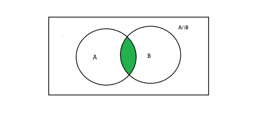
- (A
 B) is an event that occurs only when both A and B occurs.
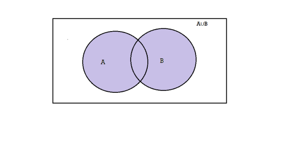
2. (A∪B) is an event that occurs when either one of A or B occurs.
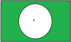
3. A’ is an event that occurs only when A does not occur.
Let S be the sample space of a random experiment and events A and B  S then
P (A  B) = P(A) + P(B) - P (A
  B)
B)
For three non-mutually exclusive events A, B and C, we have


NOTE- If events A and B are mutually exclusive events, then-
P (A  B) = P(A) + P(B)
For three mutually exclusive events A, B and C, we have
P (A  B
B ) = P(A) + P(B) + P(C)
Example: 25 lottery tickets are marked with first 25 numerals. A ticket is drawn at random. Find the probability that it is a multiple of 5 or 7.
Sol.
Let A be the event that the drawn ticket bears a number multiple of 5 and B be the event that it bears a number multiple of 7.
Therefore,
A = {5, 10, 15, 20, 25}
B = {7, 14, 21}
Here, as A 
Therefore, A and B are mutually exclusive, and hence

Example: A Card is drawn from a pack of 52 playing cards, find the probability that the drawn card is an ace or a red color card.
Sol.
Let A be the event that the drawn card is a card of ace and B be the event that it is red colour card. Now as there are four cards of ace and 26 red colour cards in a pack of 52 playing cards. Also, 2 cards in the pack are ace cards of red colour.
 and
and 
The required probability 

Mathematical expectation
Let a random variable X has a probability distribution which assumes the values say with their associated probabilities
  then the mathematical expectation can be defined as-

The expected value of a random variable X is written as E(X).
The expected value for a continuous random variable is

The mean value (μ) of the probability distribution of a variate X is commonly known as its expectation current is denoted by E (X). If f(x) is the probability density function of the variate X, then
 (Discrete distribution)
 (Continuous distribution)
In general expectation of any function is  given by
 (Discrete distribution)
 (Continuous distribution)
(2) Variance offer distribution is given by
 (Discrete distribution)
 (Continuous distribution)
Where  is the standard deviation of the distribution.
(3) The rth moment about mean (denoted by  is defined by
 (Discrete function)
 (Continuous function)
(4) Mean deviation from the mean is given by
 (Discrete distribution)
 (Continuous distribution)
Properties of expectation:
- E(k) = k, where k is a constant
- E(kX) = kE(X), k being a constant.
- E (aX + b) = aE(X) + b, where a and b are constants
Example: If a random variable X has the following probability distribution in the tabular form, then what will be the expected value of X.
X | 0 | 1 | 2 |
P(x) | 1/4 | ½ | ¼ |
Sol.
We know that-

So that-

Example: Find the expectations of the number of an unbiased die when thrown.
Sol. Let X be a random variable that represents the number on a die when thrown.
X can take the values-
1, 2, 3, 4, 5, 6
With
P [X = 1] = P [X = 2] = P [ X = 3] = P [X = 4] = P [X = 5] = P [X = 6] = 1/6
The distribution table will be-
X | 1 | 2 | 3 | 4 | 5 | 6 |
p(x) | 1/6 | 1/6 | 1/6 | 1/6 | 1/6 | 1/6 |
Hence the expectation of number on the die thrown is-

So that-

Example: If it rains, a rain coat dealer can earn Rs 500 per day. If it is a dry day, he can lose Rs 100 per day. What is his expectation, if the probability of rain is 0.4?
Sol.
Let X be the amount earned on a day by the dealer. Therefore, X can take the values Rs 500, -Rs 100
Loss of 100 Rs is equivalent to -100 Rs
| Rainy day | Dry day |
X (in Rs) | 500 | -100 |
p(x) | 0.4 | 0.6 |
Hence the expectation of the amount earned-

Thus, his expectation is Rs 140, i.e., on an overage he earns Rs 140 per day.
Example. In a lottery, m tickets are drawn at a time out of a ticket numbered from 1 to n. Find the expected value of the sum of the numbers on the tickets drawn.
Solution. Let  be the variables representing the numbers on the first, second…nth ticket. The probability of drawing a ticket out of n ticket spelling in each case 1/n, we have

Therefore, the expected value of the sum of the numbers on the tickets drawn


Variance
Variance of a random variable X is defined as the second order central moment and it is defined as-

Or

Note-
If X is a random variable, then-

Where a and b are constants.
Note-
Example: Find the following of the given probability distribution-
X | -2 | -1 | 0 | 1 | 2 |
p(x) | 0.15 | 0.30 | 0 | 0.30 | 0.25 |
- V(X)
- V (2X + 3)
Sol.
- We know that-

2. V (2X + C) = 
Key takeaways
- The mathematical expectation can be defined as-

2. The expected value for a continuous random variable is


Or

3. If X is a random variable, then-

Where a and b are constants.
A random variable is a real-valued function whose domain is a set of possible outcomes of a random experiment and range is a subset of the set of real numbers and has the following properties:
i) Each particular value of the random variable can be assigned some probability
Ii) Uniting all the probabilities associated with all the different values of the random variable gives the value 1.
A random variable is denoted by X, Y, Z, etc.
For example, if a random experiment E consists of tossing a pair of dice, the sum X of the two numbers which turn up have the value 2,3,4,…12 depending on chance. Then X is a random variable
It is a real valued function which assigns a real number to each sample point in the sample space.
A random variable X is a function defined on the sample space 5 of an experiment S of an experiment. Its value are real numbers. For every number a the probability

With which X assumes a is defined. Similarly for any interval l the probability

With which X assumes any value in I is defined.
Example:
Tossing a fair coin thrice then-
Sample Space(S) = {HHH, HHT, HTH, THH, HTT, THT, TTH, TTT}
Roll a dice
Sample Space(S) = {1,2,3,4,5,6}
A random variable is a real-valued function whose domain is a set of possible outcomes of a random experiment and range is a sub-set of the set of real numbers and has the following properties:
i) Each particular value of the random variable can be assigned some probability
Ii) Uniting all the probabilities associated with all the different values of the random variable gives the value 1.
A random variable is denoted by X, Y, Z etc.
For example if a random experiment E consists of tossing a pair of dice, the sum X of the two numbers which turn up have the value 2,3,4,…12 depending on chance. Then X is a random variable
Discrete random variable-
A random variable is said to be discrete if it has either a finite or a countable number of values. Countable number of values means the values which can be arranged in a sequence.
Note- if a random variable takes a finite set of values, it is called discrete and if a random variable takes an infinite number of uncountable values, it is called continuous variable.
Discrete probability distributions-
Let X be a discrete variate which is the outcome of some experiments. If the probability that X takes the values of x is  , then-

Where-
1. 
2. 
The set of values  with their probabilities
  makes a discrete probability distribution of the discrete random variable X.
Probability distribution of a random variable X can be exhibited as follows-
X |  |  |  |
P(x) |  |  |  |
Example: Find the probability distribution of the number of heads when three coins are tossed simultaneously.
Sol.
Let be the number of heads in the toss of three coins
The sample space will be-
{HHH, HHT, HTH, THH, HTT, THT, TTH, TTT}
Here variable X can take the values 0, 1, 2, 3 with the following probabilities-
P [X= 0] = P[TTT] = 1/8
P[X = 1] = P [HTT, THH, TTH] = 3/8
P [X = 2] = P [HHT, HTH, THH] = 3/8
P [X = 3] = P[HHH] = 1/8
Hence the probability distribution of X will be-
X |  |  |  |  |
P(x) |  |  |  |  |
Example: For the following probability distribution of a discrete random variable X,
 0 1 2 3 4 5
 0 c c 2c 3c c
Find-
1. The value of c.
2. P[1<x<4]
Sol,
1. We know that-

So that-
0 + c + c + 2c + 3c + c = 1
8c = 1
Then c = 1/8
Now, 2. P[1<x<4] = P [X = 2] + P [X = 3] = c + 2c = 3c = 3× 1/8 = 3/8
Probability density function
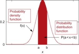
Probability density function (PDF) is an arithmetical appearance which gives a probability distribution for a discrete random variable as opposite to a continuous random variable. The difference among a discrete random variable is that we check an exact value of the variable. Like, the value for the variable, a stock worth, only goes two decimal points outside the decimal (Example 32.22), while a continuous variable have an countless number of values (Example 32.22564879…).
When the PDF is graphically characterized, the area under the curve will show the interval in which the variable will decline. The total area in this interval of the graph equals the probability of a discrete random variable happening. More exactly, since the absolute prospect of a continuous random variable taking on any exact value is zero owing to the endless set of possible values existing, the value of a PDF can be used to determine the likelihood of a random variable dropping within an exact range of values.
Example: The probability density function of a variable X is
X | 0 | 1 | 2 | 3 | 4 | 5 | 6 |
P(X) | k | 3k | 5k | 7k | 9k | 11k | 13k |
(i) Find 
(ii) What will be e minimum value of k so that 
Solution
(i) If X is a random variable then


(ii) Thus, minimum value of k=1/30.
Example: A random variate X has the following probability function
x | 0 | 1 | 2 | 3 | 4 | 5 | 6 | 7 |
P (x) | 0 | k | 2k | 2k | 3k |  |  |  |
(i) Find the value of the k.
(ii) 
Solution. (i) If X is a random variable then


(ii)


Continuous probability distribution
When a variate X takes every value in an interval it gives rise to continuous distribution of X. The distribution defined by the vidiots like heights or weights are continuous distributions.
A major conceptual difference however exists between discrete and continuous probabilities. When thinking in discrete terms the probability associated with an event is meaningful. With continuous events however where the number of events is infinitely large, the probability that a specific event will occur is practically zero. For this reason, continuous probability statements on must be worth did some work differently from discrete ones. Instead of finding the probability that x equals some value, we find the probability of x falling in a small interval.
Thus the probability distribution of a continuous variate x is defined by a function f (x) such that the probability of the variate x falling in the small interval  Symbolically it can be expressed as
  Thus f (x) is called the probability density function and then continuous curve y = f(x) is called the probability of curve.
The range of the variable may be finite or infinite. But even when the range is finite, it is convenient to consider it as infinite by opposing the density function to be zero outside the given range. Thus, if f (x) =(x) be the density function denoted for the variate x in the interval (a, b), then it can be written as


The density function f (x) is always positive and  (i.e., the total area under the probability curve and the x-axis is unity which corresponds to the requirements that the total probability of happening of an event is unity).
(2) Distribution function
If 
Then F(x) is defined as the commutative distribution function or simply the distribution function the continuous variate X. It is the probability that the value of the variate X will be ≤x. The graph of F(x) in this case is as shown in figure 26.3 (b).
The distribution function F (x) has the following properties
(i) 
(ii) 
(iii) 
(iv) P (a ≤x ≤b) =  =
=  =F (b) – F (a).
Example
(i) Is the function defined as follows a density function.

(ii) If so determine the probability that the variate having this density will fall in the interval (1.2).
(iii) Also find the cumulative probability function F (2)?
Solution. (i) f (x) is clearly ≥0 for every x in (1,2) and

Hence the function f (x) satisfies the requirements for a density function.
(ii)Required probability = 
This probability is equal to the shaded area in figure 26.3 (a).
(iii)Cumulative probability function F (2)

Which is shown in figure
Example: Show that the following function can be defined as a density function and then find  .
.


Sol.
Here

So that, the function can be defined as a density function.
Now.

Example: Let X be a continuous random variable with PDF given by

If  , find the CDF of Y.
Solution. First, we note that  , we have


Thus, 
Example: Let X be a continuous random variable with PDF

Find  .
.
Solution. We have


Key takeaways-
1. A random variable is said to be discrete if it has either a finite or a countable number of values. Countable number of values means the values which can be arranged in a sequence.
2. 
Where-
1. 
Binomial distribution
This distribution was discovered by a Swiss mathematician Jame Bernoulli (1654-1705) and is also known as Bernoulli Distribution.
The conditions for binomial distribution-
- The number of trials is finite and fixed.
- In every trial there are only two possible outcomes success or failure.
- The trials are independent. The outcome of one trial does not affect the other trial.
- p, the probability of success from trial to trial is fixed and q the probability of failure is equal to 1-p. This is the same in all the trials.
Let the probability of the happening of an event A in one trial be p and its probability of not happening be 1 – p – q.
We assume that there are n trials and the happening of the event A is r times and its not happening is n – r times.
This may be shown as follows
AA……A 
r times n – r times (1)
A indicates its happening  its failure and P (A) =p and P (
We see that (1) has the probability
Pp…p qq….q=
r times n-r times (2)
Clearly (1) is merely one order of arranging r A’S.
The probability of (1) = Number of different arrangements of r A’s and (n-r)
 ’s
’s
The number of different arrangements of r A’s and (n-r) ’s
’s 
Probability of the happening of an event r times =

If r = 0, probability of happening of an event 0 times 
If r = 1,probability of happening of an event 1 times 
If r = 2,probability of happening of an event 2 times 
If r = 3,probability of happening of an event 3 times  and so on.
These terms are clearly the successive terms in the expansion of 
Hence it is called Binomial Distribution.
Definition-
A discrete random variable X is said to be follow the binomial distribution with parameter n and p.
The probability of happening of an event r times exactly in n trials is-

Example: A die is thrown 8 times then find the probability that 3 will show-
1. Exactly 2 times
2. At least 7 times
3. At least once
Sol.
As we know that-


Then-
1. Probability of getting 3 exactly 2 times will be-

2. Probability of getting 3 at least 7 or 8 times will be-

3. Probability of getting 3 at least once or (1 or 2 or 3 or 4 or 5 or 6 or 7 or 8 times)-


Example:
If on an average one ship in every ten is wrecked. Find the probability that out of 5 ships expected to arrive, 4 at least we will arrive safely.
Solution:
Out of 10 ships one ship is wrecked.
I.e. nine ships out of 10 ships are safe, P (safety) = 
P (at least 4 ships out of 5 are safe) = P (4 or 5) = P (4) + P (5)

Example. The overall percentage of failures in a certain examination is 20. If 6 candidates appear in the examination what is the probability that at least five pass the examination?
Solution:
Probability of failures = 20% 
Probability of (P) = 
Probability of at least 5 passes = P (5 or 6)


Example:
The probability that a man aged 60 will live to be 70 is 0.65. What is the probability that out of 10 men, now 60, at least seven will live to be 70?
Solution:
The probability that a man aged 60 will live to be 70


Number of men= n = 10
Probability that at least 7 men will live to 70 = (7 or 8 or 9 or 10)
= P (7) + P (8) + P (9) + P (10) =


Example
Assuming that 20% of the population of a city are literate so that the chance of an individual being literate is  and assuming that hundred investigators each take 10 individuals to see whether they are illiterate, how many investigators would you expect to report 3 or less were literate.
Solution


Required number of investigators = 0.879126118× 100 =87.9126118
= 88 approximate
Example: The probability that an evening college student will graduate is 0.4. Determine the probability that out of 5 students (a) none, (b) one, and (c) atleast one will graduate.
Sol.
Here
n = 5, p = 0.4 or 4/10, q = 0.6 = (6/10)

(a) The probability of zero success-


(b) The probability of one success-

(c) The probability of atleast one success
= 1– probability of no success
= 1– 0.078
= 0.922
Mean and standard deviation of binomial distribution-
1. 
2. 
3. 
Moments of binomial distribution-
1. First moment about the origin-

2. Second moment about the origin-

3. Third moment about origin-

4. Fourth moment about origin-

5. Third central moment-

6. Fourth central moment-

Example: Find mean and variance of a binomial distribution with p = 1/4 and n = 10.
Sol.
Here 
Mean = np = 
Variance = npq = 
Mean or binomial distribution

Successors r | Frequency f | Rf |
0 |  | 0 |
1 |  |  |
2 |  | n(n-1)  |
3 |  |  |
….. | …… | …. |
N |  |  |


Since, 
STANDARD DEVIATION OF BINOMIAL DISTRIBUTION
Successors r | Frequency f |  |
0 |  | 0 |
1 |  |  |
2 |  | 2n(n-1)  |
3 |  |  |
….. | …… | …. |
N |  |  |
We know that  (1)
(1)
r is the deviation of items (successes) from 0.


Putting these values in (1) we have


Hence for the binomial distribution, Mean 
Example. A die is tossed thrice. A success is getting 1 or 6 on a TOSS. Find the mean and variance of the number of successes.
Solution.


RECURRENCE RELATION FOR THE BINOMIAL DISTRIBUTION
By Binomial Distribution


On dividing (2) by (1), we get


Key takeaways
1. A discrete random variable X is said to be follow the binomial distribution with parameter n and p.
The probability of happening of an event r times exactly in n trials is-

2. 
3. 
4. 
Geometric
This distribution builds upon the binomial distribution. We continue the experiment until success or failures occurs.
There are three main characteristics of geometric distribution-
1. There are one or more Bernoulli trials with all failures except the last one, which is a success. In other words, you keep repeating what you are doing until the first success.
2. The number of trials could go on forever. There must be at least one trial.
3. The probability, p, of a success and the probability, q, of a failure is the same for each trial. p+q=1 and q=1−p.
The geometric distribution represents the number of failures before you get a success in a series of Bernoulli trials.
The probability density function is given by

Mean and variance of the geometric distribution are given as-


Example: The probability of a defective TV component is 0.02. Components are randomly selected. Find the probability that the first defect is caused by the seventh component tested. How many components do you expect to test until one is found to be defective?
Sol
Let X = the number of computer components tested until the first defect is found.
X takes on the values 1, 2, 3, ... Where p = 0.02. X ~ G (0.02)
Find P(x = 7). Answer: P (x = 7) = (1 - 0.02) ^7-× 0.02 = 0.0177.
The probability that the seventh component is the first defect is 0.0177.
Uniform
Discrete uniform distribution
Definition: A random variable X is said to have a discrete uniform distribution if it takes any positive integer value from 1 to n, and its probability mass function is given by

Where n is called the parameter of the distribution.
Mean and Variance of the uniform Distribution

Example: Find the mean and variance of a number on an unbiased die when thrown.
Sol:
Suppose X be the number on an unbiased die when thrown,
Then X can take the values 1, 2, 3, 4, 5, 6 with

By uniform distribution, we have


And

Continuous uniform distribution
A random variable X is said to follow a continuous uniform distribution over an interval (a, b) if its probability density function is given by

Mean and Variance of the continuous uniform Distribution

Example: Find the coefficient of variation for the rectangular distribution in (0, 12).
Sol:
Here a = 0, b = 12


Then the SD will be-


Example: Buses are scheduled every 5 minutes at a certain bus stand. A person comes to the stand at a random time. Let the random variable X count the number of minutes he/she has to wait for the next bus. Assume X has a uniform distribution over the interval (0, 5). Find the probability that he/she has to wait at least 3 minutes for the bus.
Sol:
As X follows uniform distribution over the interval (0, 5), probability density function of X is

Thus, the desired probability

The probability that he/she has to wait at least 3 minutes for the bus is 0.4.
Chi square
When a fair coin is tossed 80 times, we expect from the theoretical considerations that heads will appear 40 times and tail 40 times. But this never happens in practice that is the results obtained in an experiment do not agree exactly with the theoretical results. The magnitude of discrepancy between observations and theory is given by the quantity  (pronounced as chi squares). If
  the observed and theoretical frequencies completely agree. As the value of
  increases, the discrepancy between the observed and theoretical frequencies increases.
Definition.
If  and
and  be the corresponding set of expected (theoretical) frequencies, then
  is defined by the relation


Chi – square distribution
If  be n independent normal variates with mean zero and s.d. Unity, then it can be shown that
  is a random variate having
  distribution with ndf.
The equation of the  curve is

(1) Properties of  distribution
- If v = 1, the
 curve (2) reduces to
  which is the exponential distribution.
 - If
 this curve is tangential to x – axis at the origin and is positively skewed as the mean is at v and mode at v-2.
 - The probability P that the value of
 from a random sample will exceed
  is given by

 have been tabulated for various values of P and for values of v from 1 to 30. (Table V Appendix 2)
 , the
, the curve approximates to the normal curve and we should refer to normal distribution tables for significant values of
  .
.
IV. Since the equation of  curve does not involve any parameters of the population, this distribution does not dependent on the form of the population.
V. Mean =  and variance =
Goodness of fit
The values of  is used to test whether the deviations of the observed frequencies from the expected frequencies are significant or not. It is also used to test how will a set of observations fit given distribution
  therefore provides a test of goodness of fit and may be used to examine the validity of some hypothesis about an observed frequency distribution. As a test of goodness of fit, it can be used to study the correspondence between the theory and fact.
This is a nonparametric distribution free test since in this we make no assumptions about the distribution of the parent population.
Procedure to test significance and goodness of fit
(i) Set up a null hypothesis and calculate

(ii) Find the df and read the corresponding values of  at a prescribed significance level from table V.
(iii) From  table, we can also find the probability P corresponding to the calculated values of
  for the given d.f.
(iv) If P<0.05, the observed value of  is significant at 5% level of significance
If P<0.01 the value is significant at 1% level.
If P>0.05, it is a good faith and the value is not significant.
Example. A set of five similar coins is tossed 320 times and the result is
Number of heads | 0 | 1 | 2 | 3 | 4 | 5 |
Frequency | 6 | 27 | 72 | 112 | 71 | 32 |
Solution. For v = 5, we have 
P, probability of getting a head=1/2; q, probability of getting a tail=1/2.
Hence the theoretical frequencies of getting 0,1,2,3,4,5 heads are the successive terms of the binomial expansion 


Thus, the theoretical frequencies are 10, 50, 100, 100, 50, 10.
Hence, 


Since the calculated value of  is much greater than
  the hypothesis that the data follow the binomial law is rejected.
Example. Fit a Poisson distribution to the following data and test for its goodness of fit at level of significance 0.05.
x | 0 | 1 | 2 | 3 | 4 |
f | 419 | 352 | 154 | 56 | 19 |
Solution. Mean m =
Hence, the theoretical frequency are 
X | 0 | 1 | 2 | 3 | 4 | Total |
F | 404.9 (406.2) | 366 | 165.4 | 49.8 | 11..3 (12.6) | 997.4 |
Hence, 

Since the mean of the theoretical distribution has been estimated from the given data and the totals have been made to agree, there are two constraints so that the number of degrees of freedom v = 5- 2=3
For v = 3, we have 
Since the calculated value of  the agreement between the fact and theory is good and hence the Poisson distribution can be fitted to the data.
Example. In experiments of pea breeding, the following frequencies of seeds were obtained
Round and yellow | Wrinkled and yellow | Round and green | Wrinkled and green | Total |
316 | 101 | 108 | 32 | 556 |
Theory predicts that the frequencies should be in proportions 9:3:3:1. Examine the correspondence between theory and experiment.
Solution. The corresponding frequencies are

Hence,


For v = 3, we have 
Since the calculated value of  is much less than
  there is a very high degree of agreement between theory and experiment.
Poisson distribution
Poisson distribution was derived in 1837 by a French mathematician Simeon D Poisson (1731-1840).
Examples of Poisson distribution-
- The number of defective articles produced by a quality machine,
- The number of persons dying due to rare disease or snake bite etc.
- The number of accidental deaths by falling from trees or roofs etc.
- The number of cars passes on road within a fixed period.
Defintion-1
Poisson distribution is a particular limiting form of the Binomial distribution when p (or q) is very small and n is large enough.
Poisson distribution is

Where m is the mean of the distribution.
Or we can define it as
Defintion-2
A random variable X is said to be follow Poisson distribution if it has the following probability mass function-


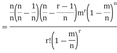
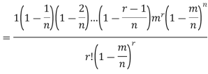
Proof. In Binomial Distribution


Taking limits when n tends to infinity


MEAN OF POISSON DISTRIBUTION

Success r | Frequency f | f.r |
0 |  | 0 |
1 |  |  |
2 |  |  |
3 |  |  |
… | … | … |
r |  |  |
… | … | … |


STANDARD DEVIATION OF POISSON DISTRIBUTION

Successive r | Frequency f | Product rf | Product  |
0 |  | 0 | 0 |
1 |  |  |  |
2 |  |  |  |
3 |  |  |  |
……. | …….. | …….. | …….. |
r |  |  |  |
…….. | ……. | …….. | ……. |


Hence mean and variance of a Poisson distribution are equal to m. Similarly we can obtain,


MEAN DEVIATION
Show that in a Poisson distribution with unit mean, and the mean deviation about the mean is 2/e times the standard deviation.
Solution
 But mean = 1 i.e. m =1 and S.D. =

r | P (r) | |r-1| | P(r)|r-1| |
0 |  | 1 |  |
1 |  | 0 | 0 |
2 |  | 1 |  |
3 |  | 2 |  |
4 |  | 3 |  |
….. | ….. | ….. | ….. |
r |  | r-1 |  |
Mean Deviation =


MOMENT GENERATING FUNCTION OF POISSON DISTRIBUTION
Solution

Let  be the moment generating function then

CUMULANTS
The cumulant generating function  is given by


Now  cumulant =coefficient of
  in K (t) = m
i.e.  , where r = 1,2,3,…
Mean = 


RECURRENCE FORMULA FOR POISSON DISTRIBUTION
SOLUTION.
By Poisson distribution


On dividing (2) by (1) we get


Applications of Poison distribution
The distribution is applied to problems concerning:
(i) Arrival pattern of defective vehicles in a workshop, patients in a hospital or telephone calls.
(ii) Demand pattern for certain spare parts.
(iii) Number of fragments from a shell hitting a target.
(iv) Spatial distribution of bomb hits.
Example. Assume that the probability of an individual coal miner being killed in a mine accident during a year is  . Use appropriate statistical distribution to calculate the probability that in a mine employing 200 miners, there will be at least one fatal accident in a year.
Solution


Example. Suppose 3% of bolts made by a machine are defective, the defects occuring at random during production. If bolts are packaged 50 per box, find
(a) Exact probability and
(b) Poisson approximation to it, that a given box will contain 5 defectives.
Solution


(a) Hence the probability for 5 defectives bolts in a lot of 50.

(b) To get Poisson approximation m = np =
Required Poisson approximation=
Example. In a certain factory producing cycle tyres, there is a smallchance of 1 in 500 tyres to be defective. The tyres are supplied in lots of 10. Using Poisson distribution, calculate the approximate number of lots containing no defective, one defective and two defective tyres, respectively, in a consignment of 10,000 lots.
Solution.


S.No. | Probability of defective | Number of lots containing defective |
1. |  |  |
2. |   |  |
3. |   |  |
Example: If cars arriving at workshop follow the Poisson distribution. If the average number of cars arrivals during a specified period of an hour is 2.
Find the probabilities that during the given hour-
1. No car arrive
2. At least two cars arrive.
Sol.
Here the average of car arrivals is - 2
So that mean = 2

Let X be the number of cars arriving during the given hour,
By using Poisson distribution, we get-

So that the required probability-
1. P [no car will arrive] = P [X = x] = 
2. P [At least two cars will arrive] = P [X≥2] = P [X =2] + P [X = 3] + ……….
= 1 - P [[X =1] + P [X =0]]


Example: If the probability that a vaccine given to the patients shows bad reaction is 0.001, then find the probability that out of 2000 patients-
1. Exactly 3 patients
2. More than 2 patients
3. No patient
Will show bad reaction.
Sol.
Here p = 0.001 and number of patients (n) = 2000
Then 
By using Poisson distribution, we get-

1. Probability that exactly 3 patients show bad reaction is-

2. Probability that more than 2 patients show bad reaction-


3. Probability that no patient shows bad reaction-

Example: If a book has 600 pages and it has 40 printing mistakes. Assume that these mistakes are randomly distributed and x the number of mistakes per page follow Poisson distribution.
What is the probability that there will not be any mistake if 10 pages selected at random?
Sol.
Here 
We get by using Poisson distribution-

Then-

Exponential Distribution:
The exponential distribution is a C.D. Which is usually used to define to come time till some precise event happens. Like, the amount of time until a storm or other unsafe weather event occurs follows an exponential distribution law.
The one-parameter exponential distribution of the probability density function PDF is defined:
f(x)=λ ,x≥0
,x≥0
Where, the rate λ signifies the
Normal amount of events in single time.
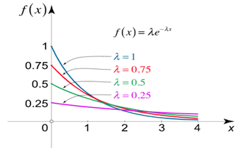
The mean value is μ=  . The median of the exponential distribution is m =
  , and the variance is shown by
  .
.
Note-
If  , then mean < Variance
If  , then mean = Variance
If  , then mean > Variance
The memoryless Property of Exponential Distribution
It can be stated as below
If X has an exponential distribution, then for every constant a  0, one has P [X
  x + a |X
  a] = P [X
  x] for all x i.e., the conditional probability of waiting up to the time 'x +a ' given that it exceeds ‘a’ is same as the probability of waiting up to the time ‘x’.
Normal distribution
The concept of normal distribution was given by English mathematician Abraham De Moivre in 1733 but the concrete theory was given by Karl Gauss that is why sometime normal distribution is called Gaussian distribution.
Normal distribution is a continuous distribution. It is derived a s the limiting form of the Binomial distribution for large values of n and p and q are not very small.
The Normal distribution is given by the equation
 …. (1)
Where =mean,  standard deviation,

On substitution  in (1), we get
  …. (2)
Here mean , standard deviation
(2) is known as standard form of normal distribution.
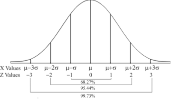
Graph of a normal probability function-
The curve looks like bell-shaped curve. The top of the bell is exactly above the mean.
If the value of standard deviation is large then curve tends to flatten out and for small standard deviation it has sharp peak.
This is one of the most important probability distributions in statistical analysis.
Mean for Normal Distribution:
Mean [Putting
  ]
]


Standard Deviation for Normal Distribution:


Put 


Median of the Normal Distribution
If a is the median, then it divides the total area into two equal halves so that,

Where 
Suppose mean,
mean,  then
then
 But
But 
 (=mean)

Thus 
Similarly, when  mean, we have
Thus, median=median .
.
Mean Deviation about the Mean
Mean Deviation 

 where
where 

 (As the function is given)
 approximately.
Mode of the Normal distribution
We know that mode is the value of the variate x for which  is maximum. Thus, by differential calculus
  is maximum if
  and
and 
Where 
Clearly will be maximum when the exponent will be maximum which will be the when
Thus, mode is and modal ordinate 
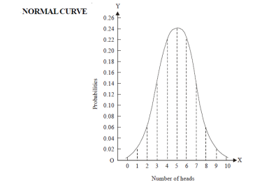
Let us show binomial distribution graphically. The probabilities of heads in 1 toss are 

 . It is shown in the given figure.
If the variates (heads here) are treated as if they were continuous, the required probability curve will be a normal curve as shown in the above figure by dotted lines.
Properties of the normal curve:
- The curve is symmetrical about the y – axis. The mean, median and mode coincide at the origin.
- The curve is drawn, if mean (origin of x) and standard deviation are given. The value of
 can be calculated from the fact that the area of the curve must be equal to the total number of observations.
 - Y decreases rapidly as
 increases numericallu. The curve extends to infinity on either side of the origin.
4.
(a) 
(b)
(c) 
Hence (a) About  of the values will lie between
  and
and .
.
(b) About 95% of the values will lie between  and
and .
.
(c) About 99.7% of the values will lie between  and
and .
.
Area under the Normal curve
By taking  , the standard normal curve is formed.
The total area under this curve is 1. The area under the curve is divided into two equal parts by . Left hand side are and right-hand side area to
  is
is  . The area between the ordinate
 .
.
Example:
1. If X  then find the probability density function of X.
2. If X  then find the probability density function of X.
Sol.
1. We are given X 
Here 
We know that-

Then the p.d.f. will be-

2. We are given X 
Here 
We know that-

Then the p.d.f. will be-

Example. X is a normal variate with mean 30 and S.D. 5, find the probabilities that
(i) 
(ii) 
(iii) |X-30|≥5
Solution. We have μ =30 and  =5
=5

(i) When X = 26,z = -0.8, when X =40, z =-2


(ii) When X =45, z =3


(iii) 


Example:
In a normal distribution 31% of the items are under 45 and 8% are over 64. Find the mean and standard deviation of the distribution.
Solution.
Let  be the mean and
  the standard deviation 31% of the items are under 45 means area to the left of the ordinate x = 45
When x = 45, let z 


From table III 
When x = 64, let  so that
Hence, 
From table III 
From (i) and (ii), 
From (iii) and (iv), 
Solving these equations, we get 
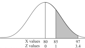
Example: If a random variable X is normally distributed with mean 80 and standard deviation 5, then find-
1. P[X > 95]
2. P[X < 72]
3. P [85 < X <97]
[Note- use the table- area under the normal curve]
Sol.
The standard normal variate is – 
Now-
1. X = 95,

So that-


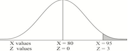
2. X = 72,

So that-


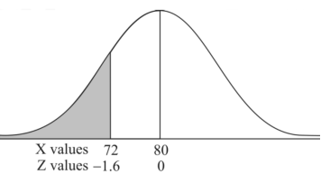
3. X = 85,

X = 97,

So that-


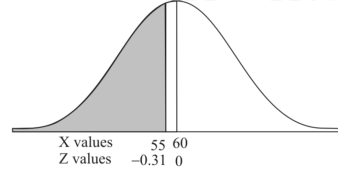
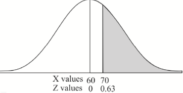
Example: In a company the mean weight of 1000 employees is 60kg and standard deviation is 16kg.
Find the number of employees having their weights-
1. Less than 55kg.
2. More than 70kg.
3. Between 45kg and 65kg.
Sol. Suppose X be a normal variate = the weight of employees.
Here mean 60kg and S.D. = 16kg
X 
Then we know that-

We get from the data,

Now-
1. For X = 55,

So that-


2. For X = 70,

So that-

3. For X = 45,

For X = 65,


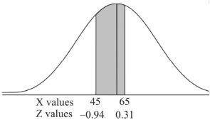
Hence the number of employees having weights between 45kg and 65kg-

Example: The mean inside diameter of a sample of 200 washers produced by a machine is 0.0502 cm and the standard deviation is 0.005 cm. The purpose for which these washers are intended allows a maximum tolerance in the diameter of 0.496 to 0.508 cm, otherwise the washers are considered defective. Determine the percentage of defective washers produced by the machine, assuming the diameters are normally distributed.
Sol.
Here-

And

Area for non-defective washers = area between z = -1.2 to +1.2
= 2 area between z = 0 and z = 1.2
= 2 × 0.3849 = 0.7698 = 76.98%
Then percent of defective washers = 100 – 76.98 = 23.02 %
Example: The life of electric bulbs is normally distributed with mean 8 months and standard deviation 2 months.
If 5000 electric bulbs are issued how many bulbs should be expected to need replacement after 12 months?
[Given that P (z ≥ 2) = 0. 0228]
Sol.
Here mean (μ) = 8 and standard deviation = 2
Number of bulbs = 5000
Total months (X) = 12
We know that-

Area (z ≥ 2) = 0.0228
Number of electric bulbs whose life is more than 12 months (Z> 12)
= 5000 × 0.0228 = 114
Therefore, replacement after 12 months = 5000 – 114 = 4886 electric bulbs.
Key takeaways
- The Normal distribution is given by the equation

Median=median .
.
2. The curve is symmetrical about the y – axis. The mean, median and mode coincide at the origin.
3. The curve is drawn, if mean (origin of x) and standard deviation are given. The value of can be calculated from the fact that the area of the curve must be equal to the total number of observations.
4. Y decreases rapidly as  increases numericallu. The curve extends to infinity on either side of the origin.
5. (a) 
(b)
(c) 
Rank of a matrix by echelon form-
The rank of a matrix (r) can be defined as –
1. It has at least one non-zero minor of order r.
2. Every minor of A of order higher than r is zero.
Example: Find the rank of a matrix M by echelon form.
M = 
Sol. First we will convert the matrix M into echelon form,
M = 
Apply,  , we get
M = 
Apply  , we get
M = 
Apply 
M = 
We can see that, in this echelon form of matrix, the number of non – zero rows are 3.
So that the rank of matrix X will be 3.
Example: Find the rank of a matrix A by echelon form.
A = 
Sol. Convert the matrix A into echelon form,
A = 
Apply 
A = 
Apply  , we get
A = 
Apply  , we get
A = 
Apply  ,
,
A = 
Apply  ,
,
A = 
Therefore, the rank of the matrix will be 2.
Example: Find the rank of a matrix A by echelon form.
A = 
Sol. Transform the matrix A into echelon form, then find the rank,
We have,
A = 
Apply, 
A = 
Apply  ,
,
A = 
Apply 
A = 
Apply 
A = 
Hence the rank of the matrix will be 2.
Example: Find the rank of the following matrices by echelon form?
Let A = 
Applying 
A 
Applying 
A 
Applying 
A 
Applying 
A 
It is clear that minor of order 3 vanishes but minor of order 2 exists as 
Hence rank of a given matrix A is 2 denoted by 
2. 
Let A = 
Applying 

Applying 

Applying 

The minor of order 3 vanishes but minor of order 2 non zero as 
Hence the rank of matrix A is 2 denoted by 
3. 
Let A = 
Apply 

Apply 

Apply 

It is clear that the minor of order 3 vanishes whereas the minor of order 2 is non zero as 
Hence the rank of given matrix is 2 i.e., 
Rank of a matrix by normal form-
Any matrix ‘A’ which is non-zero can be reduced to a normal form of ‘A’ by using elementary transformations.
There are 4 types of normal forms –

The number r obtained is known as rank of matrix A.
Both row and column transformations may be used in order to find the rank of the matrix.
Note-Normal form is also known as canonical form
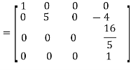
Example: reduce the matrix A to its normal form and find rank as well.

Sol. We have,

We will apply elementary row operation,


We get,

Now apply column transformation,


We get,

Apply
 , we get,

Apply  and
and 
Apply 

Apply  and
and 


Apply  and
and 

As we can see this is required normal form of matrix A.
Therefore, the rank of matrix A is 3.
Example: Find the rank of a matrix A by reducing into its normal form.

Sol. We are given,

Apply


Apply


This is the normal form of matrix A.
So that the rank of matrix A = 3
Solution of system of linear equations-consistency
There are two types of linear equations-
1. Consistent
2. Inconsistent
Let’s understand about these two types of linear equations.
Consistent –
If a system of equations has one or more than one solution, it is said be consistent.
There could be unique solution or infinite solution.
For example-
A system of linear equations-
2x + 4y = 9
x + y = 5
Has unique solution,
Whereas,
A system of linear equations-
2x + y = 6
4x + 2y = 12
Has infinite solutions.
Inconsistent-
If a system of equations has no solution, then it is called inconsistent.
Consistency of a system of linear equations-
Suppose that a system of linear equations is given as-


This is the format as AX = B
Its augmented matrix is-
[A: B] = C
(1) Consistent equations-
If Rank of A = Rank of C
Here, Rank of A = Rank of C = n (no. Of unknown) – unique solution
And Rank of A = Rank of C = r, where r<n - infinite solutions
(2) Inconsistent equations-
If Rank of A ≠ Rank of C
Solution of homogeneous system of linear equations-
A system of linear equations of the form AX = O is said to be homogeneous, where A denotes the coefficients and of matrix and O denotes the null vector.
Suppose the system of homogeneous linear equations is,


It means
AX = O
Which can be written in the form of matrix as below,

Note- A system of homogeneous linear equations always has a solution if
1. r(A) = n then there will be trivial solution, where n is the number of unknown,
2. r(A) < n, then there will be an infinite number of solutions.
Example: Find the solution of the following homogeneous system of linear equations,


Sol. The given system of linear equations can be written in the form of matrix as follows,

Apply the elementary row transformation,


 , we get,


 , we get

Here r(A) = 4, so that it has trivial solution,

Example: Find out the value of ‘b’ in the system of homogeneous equations-
2x + y + 2z = 0
x + y + 3z = 0
4x + 3y + bz = 0
Which has
(1) Trivial solution
(2) Non-trivial solution
Sol. (1)
For trivial solution, we already know that the values of x, y and z will be zero, so that ‘b’ can have any value.
Now for non-trivial solution-
(2)
Convert the system of equations into matrix form-
AX = O

Apply  Respectively, we get the following resultant matrices


For non-trivial solutions, r(A) = 2 < n
b – 8 = 0
b = 8
Solution of non-homogeneous system of linear equations-
Example-1: check whether the following system of linear equations is consistent of not.
2x + 6y = -11
6x + 20y – 6z = -3
6y – 18z = -1
Sol. Write the above system of linear equations in augmented matrix form,

Apply  , we get

Apply 

Here the rank of C is 3 and the rank of A is 2
Therefore, both ranks are not equal. So that the given system of linear equations is not consistent.
Example: Check the consistency and find the values of x, y and z of the following system of linear equations.
2x + 3y + 4z = 11
X + 5y + 7z = 15
3x + 11y + 13z = 25
Sol. Re-write the system of equations in augmented matrix form.
C = [A, B]
That will be,

Apply 

Now apply,
We get,
 ~
~ ~
~
Here rank of A = 3
And rank of C = 3, so that the system of equations is consistent,
So that we can solve the equations as below,
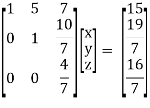
That gives,
x + 5y + 7z = 15 ……………..(1)
y + 10z/7 = 19/7 ………………(2)
4z/7 = 16/7 ………………….(3)
From eq. (3)
z = 4,
From 2,

From eq. (1), we get
x + 5(-3) + 7(4) = 15
That gives,
x = 2
Therefore, the values of x, y, z are 2, -3, 4 respectively.
Characteristic equation:-
Let A he a square matrix,  be any scalar then
  is called characteristic equation of a matrix A.
Note:
Let a be a square matrix and ‘ ’ be any scalar then,
1)  is called characteristic matrix
2)  is called characteristic polynomial.
The roots of a characteristic equations are known as characteristic root or latent roots, Eigen values or proper values of a matrix A.
Eigen vector:-
Suppose  be an Eigen value of a matrix A. Then
  a non – zero vector x1 such that.
 … (1)
… (1)
Such a vector ‘x1’ is called as Eigen vector corresponding to the Eigen value  .
.
Properties of Eigen values:-
- Then sum of the Eigen values of a matrix A is equal to sum of the diagonal elements of a matrix A.
- The product of all Eigen values of a matrix A is equal to the value of the determinant.
- If
 are n Eigen values of square matrix A then
  are m Eigen values of a matrix A-1.
 - The Eigen values of a symmetric matrix are all real.
- If all Eigen values are non –zero then A-1 exist and conversely.
- The Eigen values of A and A’ are same.
Properties of Eigen vector:-
- Eigen vector corresponding to distinct Eigen values are linearly independent.
- If two are more Eigen values are identical then the corresponding Eigen vectors may or may not be linearly independent.
- The Eigen vectors corresponding to distinct Eigen values of a real symmetric matrix are orthogonal.
Example1: Find the sum and the product of the Eigen values of  ?
?
Sol. The sum of Eigen values = the sum of the diagonal elements
 =1+(-1) =0
The product of the Eigen values is the determinant of the matrix

On solving above equations, we get 
Example2: Find out the Eigen values and Eigen vectors of  ?
?
Sol. The Characteristics equation is given by 


Or 
Hence the Eigen values are 0,0 and 3.
The Eigen vector corresponding to Eigen value  is
is

Where X is the column matrix of order 3 i.e.

This implies that 
Here number of unknowns are 3 and number of equation is 1.
Hence, we have (3-1) = 2 linearly independent solutions.
Let 
Thus, the Eigen vectors corresponding to the Eigen value  are (-1,1,0) and (-2,1,1).
The Eigen vector corresponding to Eigen value  is
is

Where X is the column matrix of order 3 i.e.

This implies that 


Taking last two equations we get

Or 
Thus, the Eigen vectors corresponding to the Eigen value  are (3,3,3).
Hence the three Eigen vectors obtained are (-1,1,0), (-2,1,1) and (3,3,3).
Example3: Find out the Eigen values and Eigen vectors of 
Sol. Let A =
The characteristics equation of A is  .
.


Or 
Or 
Or 
Or 
The Eigen vector corresponding to Eigen value  is
is

Where X is the column matrix of order 3 i.e.

Or 


On solving we get 
Thus, the Eigen vectors corresponding to the Eigen value  is (1,1,1).
The Eigen vector corresponding to Eigen value  is
is

Where X is the column matrix of order 3 i.e.

Or 


On solving  or
or  .
.
Thus, the Eigen vectors corresponding to the Eigen value  is (0,0,2).
The Eigen vector corresponding to Eigen value  is
is

Where X is the column matrix of order 3 i.e.

Or 


On solving we get  or
or  .
.
Thus, the Eigen vectors corresponding to the Eigen value  is (2,2,2).
Hence three Eigen vectors are (1,1,1), (0,0,2) and (2,2,2).
Example-4:
Determine the Eigen values of Eigen vector of the matrix.

Solution:
Consider the characteristic equation as, 
i.e. 
i.e. 


i.e. 
Which is the required characteristic equation.


 are the required Eigen values.
Now consider the equation
 … (1)
… (1)
Case I:
If  Equation (1) becomes

R1 + R2


Thus 
 independent variable.
Now rewrite equation as,


Put x3 = t
 &
&


Thus  .
.
Is the eigen vector corresponding to  .
.
Case II:
If  equation (1) becomes,


Here 
 Independent variables
Now rewrite the equations as,


Put 
 &
&


 .
.
Is the eigen vector corresponding to  .
.
Case III:
If  equation (1) becomes,


Here rank of 
 independent variable.
Now rewrite the equations as,


Put 

Thus  .
.
Is the eigen vector for  .
.
Example-5:
Find the Eigen values of Eigen vector for the matrix.

Solution:
Consider the characteristic equation as 
i.e. 


i.e. 


 are the required eigen values.
Now consider the equation
 … (1)
… (1)
Case I:
 Equation (1) becomes,


Thus  and n = 3
 3 – 2 = 1 independent variables.
Now rewrite the equations as,


Put 
 ,
, 

i.e.
The Eigen vector for 
Case II:
If  equation (1) becomes,


Thus 

Independent variables.
Now rewrite the equations as,


Put 


Is the Eigen vector for
Now
Case III:-
If  equation (1) gives,

R1 – R2


Thus 

Independent variables
Now 

Put 
Thus

Is the Eigen vector for
Key takeaways-
- Let A he a square matrix,
 be any scalar then
  is called characteristic equation of a matrix A.
 - If two are more Eigen values are identical then the corresponding Eigen vectors may or may not be linearly independent.
- The Eigen vectors corresponding to distinct Eigen values of a real symmetric matrix are orthogonal
Symmetric matrix:
In linear algebra, a symmetric matrix is a square matrix that is equal to its transpose. Formally, because equal matrices have equal dimensions, only square matrices can be symmetric. The entries of a symmetric matrix are symmetric with respect to the main diagonal. So, if aᵢⱼ denotes the entry in the i-th row and j-th column then for all indices i and j. Every square diagonal matrix is symmetric, since all off-diagonal elements are zero.
Any square matrix is said to be symmetric matrix if its transpose equals to the matrix itself.
For example:
 &
& 
Example: check whether the following matrix A is symmetric or not?
A = 
Sol. As we know that if the transpose of the given matrix is same as the matrix itself then the matrix is called symmetric matrix.
So that, first we will find its transpose,
Transpose of matrix A,

Here,
A = 
So that, the matrix A is symmetric.
Example: Show that any square matrix can be expressed as the sum of symmetric matrix and anti- symmetric matrix.
Sol. Suppose A is any square matrix.
Then,
A = 
Now,
(A + A’)’ = A’ + A
A+A’ is a symmetric matrix.
Also,
(A - A’)’ = A’ – A
Here A’ – A is an anti – symmetric matrix
So that,
Square matrix = symmetric matrix + anti-symmetric matrix
Example: Let us test whether the given matrices are symmetric or not i.e., we check for,
A = 
(1) A = 
Now
 =
=
 A =
A = 
Hence the given matric symmetric
Example: let A be a real symmetric matrix whose diagonal entries are all positive real numbers.
Is this true for all of the diagonal entries of the inverse matrix A-1 are also positive? If so, prove it. Otherwise give a counter example
Solution: The statement is false, hence we give a counter example
Let us consider the following 2 2 matrix
A = 
The matrix A satisfies the required conditions, that is A is symmetric and its diagonal entries are positive.
The determinant det(A) = (1)(1)-(2)(2) = -3 and the inverse of A is given by
A-1=  =
= 
By the formula for the inverse matrix for 2 2 matrices.
This shows that the diagonal entries of the inverse matric A-1 are negative.
Skew-symmetric:
A skew-symmetric matrix is a square matrix that is equal to the negative of its own transpose. Anti-symmetric matrices are commonly called as skew-symmetric matrices.
In other words-
Skew-symmetric matrix-
A square matrix A is said to be skew Symmetrix matrix if –
1. A’ = -A, [ A’ is the transpose of A]
2. All the main diagonal elements will always be zero.
For example-
A = 
This is skew symmetric matrix, because transpose of matrix A is equals to negative A.
Example: check whether the following matrix A is symmetric or not?
A = 
Sol. This is not a skew symmetric matrix, because the transpose of matrix A is not equals to -A.
-A = A’
Example: Let A and B be n n skew-matrices. Namely AT = -A and BT = -B
(a) Prove that A+B is skew-symmetric.
(b) Prove that cA is skew-symmetric for any scalar c.
(c) Let P be an m n matrix. Prove that PTAP is skew-symmetric.
Solution: (a) (A+B)T = AT + BT = (-A) +(-B) = -(A+B)
Hence A+B is skew symmetric.
(b) (cA)T = c.AT =c(-A) = -cA
Thus, cA is skew-symmetric.
(c)Let P be an m n matrix. Prove that PT AP is skew-symmetric.
Using the properties, we get,
(PT AP)T = PTAT(PT)T = PTATp
= PT (-A) P = - (PT AP)
Thus (PT AP) is skew-symmetric.
Diagonalisation of Matrices
Two square matrix  and A of same order n are said to be similar if and only if
 for some non-singular matrix P.
Such transformation of the matrix A into  with the help of non-singular matrix P is known as similarity transformation.
Similar matrices have the same Eigen values.
If X is an Eigen vector of matrix A, then  is Eigen vector of the matrix
Reduction to Diagonal Form:
Let A be a square matrix of order n has n linearly independent Eigen vectors Which form the matrix P such that

Where P is called the modal matrix and D is known as spectral matrix.
Procedure: let A be a square matrix of order 3.
Let three Eigen vectors of A are  Corresponding to Eigen values
Let

 {by characteristics equation of A}
Or 
Or 
Note: The method of diagonalization is helpful in calculating power of a matrix.
 .Then for an integer n we have
We are using the example of 1.6*
Example1: Diagonalise the matrix 
Let
A= 
The three Eigen vectors obtained are (-1,1,0), (-1,0,1) and (3,3,3) corresponding to Eigen values  .
.
Then

And

Also, we know that 


Example2: Diagonalise the matrix
Let A =
The Eigen vectors are (4,1), (1, -1) corresponding to Eigen values  .
.
Then  and also
Also, we know that 


Key takeaways-
- Two square matrix
 and A of same order n are said to be similar if and only if
 for some non-singular matrix P.
2. If X is an Eigen vector of matrix A, then  is Eigen vector of the matrix
3. Any square matrix is said to be symmetric matrix if its transpose equals to the matrix itself.
4. Square matrix = symmetric matrix + anti-symmetric matrix
5. A skew-symmetric matrix is a square matrix that is equal to the negative of its own transpose. Anti-symmetric matrices are commonly called as skew-symmetric matrices.
References:
- E. Kreyszig, “Advanced Engineering Mathematics”, John Wiley & Sons, 2006.
- P. G. Hoel, S. C. Port and C. J. Stone, “Introduction to Probability Theory”, Universal Book Stall, 2003.
- S. Ross, “A First Course in Probability”, Pearson Education India, 2002.
- W. Feller, “An Introduction to Probability Theory and Its Applications”, Vol. 1, Wiley, 1968.
- N.P. Bali and M. Goyal, “A Text Book of Engineering Mathematics”, Laxmi Publications, 2010.
- B.S. Grewal, “Higher Engineering Mathematics”, Khanna Publishers, 2000.
- T. Veerarajan, “Engineering Mathematics”, Tata Mcgraw-Hill, New Delhi, 2010
- Higher engineering mathematics, HK Dass
- Higher engineering mathematics, BV Ramana.
- Computer based numerical & statistical techniques, M goyal


