UNIT–3 | unit 3 probability distribution

UNIT–3

Probability Distribution

3.1. Random variable

A random variable is a real-valued function whose domain is a set of possible outcomes of a random experiment and range is a sub-set of the set of real numbers and has the following properties:

i) Each particular value of the random variable can be assigned some probability

Ii) Uniting all the probabilities associated with all the different values of the random variable gives the value 1.

A random variable is denoted by X, Y, Z etc.

For example if a random experiment E consists of tossing a pair of dice, the sum X of the two numbers which turn up have the value 2,3,4,…12 depending on chance. Then X is a random variable

Discrete random variable-

A random variable is said to be discrete if it has either a finite or a countable number of values. Countable number of values means the values which can be arranged in a sequence.

Note- if a random variable takes a finite set of values it is called discrete and if if a random variable takes an infinite number of uncountable values it is called continuous variable.

Discrete probability distributions-

Let X be a discrete variate which is the outcome of some experiments. If the probability that X takes the values of x is , then-

Where-

The set of values with their probabilities makes a discrete probability distribution of the discrete random variable X.

Probability distribution of a random variable X can be exhibited as follows-

and so on

P(x)

Example: Find the probability distribution of the number of heads when three coins are tossed simultaneously.

Sol.

Let be the number of heads in the toss of three coins

The sample space will be-

{HHH, HHT, HTH, THH, HTT, THT, TTH, TTT}

Here variable X can take the values 0, 1, 2, 3 with the following probabilities-

P[X= 0] = P[TTT] = 1/8

P[X = 1] = P [HTT, THH, TTH] = 3/8

P[X = 2] = P[HHT, HTH, THH] = 3/8

P[X = 3] = P[HHH] = 1/8

Hence the probability distribution of X will be-

P(x)

Example: For the following probability distribution of a discrete random variable X,

Find-

1. The value of c.

2. P[1<x<4]

Sol,

1. We know that-

So that-

0 + c + c + 2c + 3c + c = 1

8c = 1

Then c = 1/8

Now, 2. P[1<x<4] = P[X = 2] + P[X = 3] = c + 2c = 3c = 3× 1/8 = 3/8

Continuous probability distribution n-

When a random variable X takes every value in an interval, it gives to continuous distribution of X.

The probability distribution of a continuous variate x defined by a function f(x) such that the probabilities of the variate x falling in the interval

We express it as-

Here f(x) is called the probability density function.

Distribution function-

If F(x) = P(X≤x) = then F(x) is called as the distribution function of X.

It has the following properties-

1. F(-∞) = 0

2. F(∞) = 1

Example: Show that the following function can be defined as a density function and then find .

Sol.

Here

So that, the function can be defined as a density function.

Now.

3.2. Binomial distribution

Where-

The set of values with their probabilities constitute a discrete probability distribution of the discrete variable X.

Binomial distribution-

A discrete random variable X is said to be follow the binomial distribution with parameter n and p.

The probability of happening of an event r times exactly in n trials is-

Example: A die is thrown 8 times then find the probability that 3 will show-

1. Exactly 2 times

2. At least 7 times

3. At least once

Sol.

As we know that-

Then-

1. Probability of getting 3 exactly 2 times will be-

2. Probability of getting 3 at least 7 or 8 times will be-

3. Probability of getting 3 at least once or (1 or 2 or 3 or 4 or 5 or 6 or 7 or 8 times)-

Example: If the percentage of failure in a test is 20. If six students appear in the test, then what will be the probability that at least five students will pass the test?

Sol.

Here

Then the probability of at least five students will pass the test-

Mean and standard deviation of binomial distribution-

Moments of binomial distribution-

1. First moment about the origin-

2. Second moment about the origin-

3. Third moment about origin-

4. Fourth moment about origin-

5. Third central moment-

6. Fourth central moment-

Example: Find mean and variance of a binomial distribution with p = 1/4 and n = 10.

Sol.

Here

Mean = np =

Variance = npq =

Example: If a dice is rolled thrice. A success is getting 1 or 6 on a roll. Find the mean variance of the number of success.

Sol.

Here n = 3 , p = 1/3 and q = 2/3

Mean = np = 1

And variance = npq = 2/3

3.3. Poisson distribution

Poisson distribution is a limiting case of binomial distribution under certain conditions listed below-

1. n, the number of trials are infinitely large.

2. p, the probability of success for each trial is very small.

3. Np is finite quantity say

A random variable X is said to be follow Poisson distribution if it has the following probability mass function-

Moments of Poisson distribution-

1. First moment about origin- which Is known as mean.

2. Second moment about origin-

3. Third moment about origin-

4. Fourth moment about origin-

Note-

1. Poisson distribution is always positively skewed distribution.

2. Mean and variance of Poisson dist. Are always equal

For Poisson distribution-

Example: If cars arriving at workshop follow the Poisson distribution. If the average number of cars arrivals during a specified period of an hour is 2.

Find the probabilities that during the given hour-

1. No car arrive

2. At least two cars arrive.

Sol.

Here the average of car arrivals is - 2

So that mean = 2

Let X be the number of cars arriving during the given hour,

By using Poisson distribution, we get-

So that the required probability-

1. P [no car will arrive] = P [X = x] =

2. P [At least two cars will arrive] = P [X≥2] = P [X =2] + P [X = 3] + ……….

= 1 - P [[X =1] + P [X =0]]

Example: If the probability that a vaccine given to the patients shows bad reaction is 0.001, then find the probability that out of 2000 patients-

1. Exactly 3 patients

2. More than 2 patients

3. No patient

Will show bad reaction.

Sol.

Here p = 0.001 and number of patients (n) = 2000

Then

By using Poisson distribution, we get-

1. Probability that exactly 3 patients show bad reaction is-

2. Probability that more than 2 patients show bad reaction-

3. Probability that no patient shows bad reaction-

Example: If a book has 600 pages and it has 40 printing mistakes. Assume that these mistakes are randomly distributed and x the number of mistakes per page follow Poisson distribution.

What is the probability that there will not be any mistake if 10 pages selected at random?

Sol.

Here

We get by using Poisson distribytion-

Then-

3.4. Normal distribution

The concept of normal distribution was given by English mathematician Abraham De Moivre in 1733 but the concrete theory was given by Karl Gauss that is why sometime normal distribution is called Gaussian distribution.

Normal distribution is a continuous distribution. It is a limiting case of binomial distribution.

The probability density function of a normal distribution is given by-

Here

Where

Note-

1. If a random variable X follows normal distribution with mean and variance then we can write it as- X

2. If X , then is called standard normal variate with mean 0 and standard deviation 1.

3. The probability density function of standard normal variate Z is given as-

Where

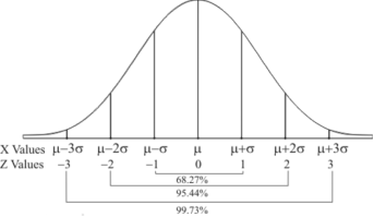
Graph of a normal probability function-

The curve look like bell-shaped curve. The top of the bell is exactly above the mean.

If the value of standard deviation is large then curve tends to flatten out and for small standard deviation it has sharp peak.

This is one of the most important probability distributions in statistical analysis.

Example:

1. If X then find the probability density function of X.

2. If X then find the probability density function of X.

Sol.

1. We are given X

Here

We know that-

Then the p.d.f. will be-

2. We are given X

Here

We know that-

Then the p.d.f. will be-

Mean, median and mode of the normal distribution-

Let ‘a’ is the median, then it divides the total area into two parts-

Where-

Let a>mean, then-

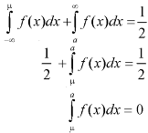
Thus-

So that mean = median.

Note- mean deviation about mean is =

Mode-

The mode of the normal distribution is and modal ordinate is given by-

Hence the mean, median and mode are equal in normal distribution.

Area property of a normal distribution (Area under the normal curve)-

Let X follows the normal distribution with mean and variance

We form a normal curve by taking

Note- Total area under the curve is always 1.

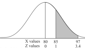
Example: If a random variable X is normally distributed with mean 80 and standard deviation 5, then find-

1. P[X > 95]

2. P[X < 72]

3. P [85 < X <97]

[Note- use the table- area under the normal curve]

Sol.

The standard normal variate is –

Now-

1. X = 95,

So that-

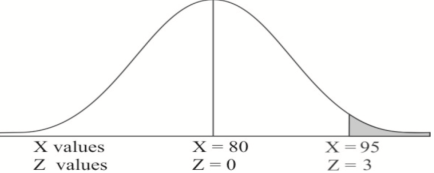
2. X = 72,

So that-

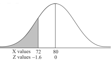
3. X = 85,

X = 97,

So that-

Example: In a company the mean weight of 1000 employees is 60kg and standard deviation is 16kg.

Find the number of employees having their weights-

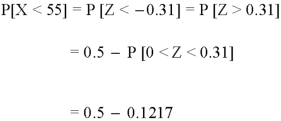
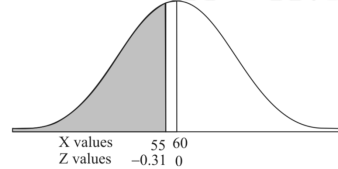
1. Less than 55kg.

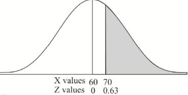
2. More than 70kg.

3. Between 45kg and 65kg.

Sol. Suppose X be a normal variate = the weight of employees.

Here mean 60kg and S.D. = 16kg

Then we know that-

We get from the data,

Now-

1. For X = 55,

So that-

2. For X = 70,

So that-

3. For X = 45,

For X = 65,

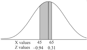
Hence the number of employees having weights between 45kg and 65kg-

Example: The mean inside diameter of a sample of 200 washers produced by a machine is 0.0502 cm and the standard deviation is 0.005 cm. The purpose for which these washers are intended allows a maximum tolerance in the diameter of 0.496 to 0.508 cm, otherwise the washers are considered defective. Determine the percentage of defective washers produced by the machine, assuming the diameters are normally distributed.

Sol.

Here-