Unit -6
Business Intelligence and Data Warehouses
Organizations grow and prosper as they gain a far better understanding of their environment. Most managers ready to track daily transactions to judge how the business is performing. By tapping into the operational database, management can develop strategies to satisfy organizational goals.
Additionally, data analysis can provide information about short-term tactical evaluations and methods like these: Are our advertisements working? What market percentage are we controlling? Are we attracting new customers? Tactical and strategic decisions shaped by constant pressure from external and internal forces, with globalization, the cultural and legal environment, and technology.
There are various competitive pressures, managers are always trying to find a competitive advantage through product development and maintenance, service, market positioning, advertisement, and so on. Managers understand that the business climate is dynamic therefore mandates their prompt reaction to vary so as to stay competitive.
Additionally, the modern business climate requires managers to approach increasingly complex problems that involve a rapidly growing number of internal and external variables. It should also come as no surprise that interest is growing in creating support systems dedicated to facilitating quick decision making during a complex environment.
Different managerial levels require different decision support needs. For instance, transaction-processing systems, supported operational databases, are tailored to serve the information needs of individuals who affect short-term inventory, accounts payable, and buying.
Middle-level managers, general managers, vice presidents, and presidents focus on strategic and tactical decision making. Those managers require detailed information designed to assist them make decisions during a complex data and analysis environment.
Companies and software vendors addressed these multilevel decision support needs by creating independent applications to fit the requirements of particular areas such as finance, customer management, human resources. Applications were also tailored to different industry sectors like education, retail, health care, or financial. This approach worked well for a few time, but changes within the business world involved new ways of integrating and managing data across levels, sectors, and geographic locations. This more comprehensive and integrated decision support framework within organizations became referred to as business intelligence.
Business intelligence (BI) describe a comprehensive, cohesive, and integrated set of tools and processes used to capture, collect, integrate, store, and analyze data with the aim of generating and presenting information used to support business decision making. Because the names implies, BI is creating intelligence a few business. This intelligence is predicated on learning and understanding the facts a few business environments.
BI is a framework that permits a business to transform data into information, information into knowledge, and knowledge into wisdom. BI has the potential to positively affect a company’s culture by creating “business wisdom” and distributing it to all or any users in an organization. This business wisdom empowers users to form business decisions supported the accumulated knowledge of the business as reflected on recorded facts. Following table shows some real-world samples of companies that have implemented BI tools and shows how the use of such tools benefited the companies.
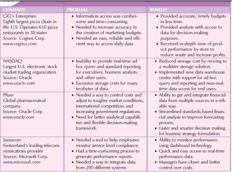
Figure 6.2(I) shows solving business problems and adding value with BI tools
BI may be a comprehensive endeavor because it encompasses all business processes within an organization. Business processes are the central units of operation during a business. Implementing BI in an organization involves capturing not only business data but also the metadata that means data about the data. BI is a complex proposition that needs an understanding and alignment of the business processes, the internal and external data, and therefore the information needs of users in the least levels in an organization.
BI isn't a product by itself, but a framework of concepts, practices, tools, and technologies which help a business understand its core capabilities, provide snapshots of the company situation, and identify opportunities to make competitive advantage. BI provides a well-orchestrated framework for the management of data that works across all levels of the organization. BI contains the following general steps:
1. Collecting and storing operational data.
2. Aggregating the operational data into decision support data.
3. Analyzing decision support data to get information.
4. Represent these information to the end user to support business decisions.
5. Making business decisions, which successively generate more data that's collected, stored, etc.
6. Monitoring results to judge outcomes of the business decisions to provide more data to be collected, stored.
To implement all above steps, BI uses many components and technologies.
BI covers a variety of technologies and applications to manage the whole data life cycle from acquisition to storage, transformation, integration, analysis, monitoring, presentation, and archiving. BI functionality is from simple data gathering and extraction to very complex data analysis and presentation. There’s no single BI architecture and it ranges from highly integrated applications from one vendor to a loosely integrated, multivendor environment. Therefore, there are some general forms of functionality that each one BI implementations share.
Like any critical business IT infrastructure, the BI architecture consists of data, people, processes, technology, and therefore the management of such components. Figure shows how all those components fit together within the BI framework.
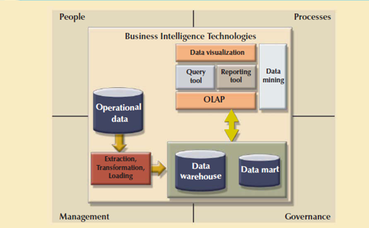
Figure 6.3(I) shows Business development architecture
Remember that the most focus of BI is to collect, integrate, and store business data for the aim of making information. BI integrates people and processes using technology so as to add value to the business. Such value is derived from how end users use such information in their daily activities, and especially, their daily business decision making.
The focus of traditional information systems was on operational automation and reporting and BI tools focus on the strategic and tactical use of data. To achieve this goal, BI recognizes that technology alone isn't enough. Therefore, BI uses an arrangement of the simplest management practices to manage data as a company asset. One among the most recent developments during this area is that the use of master data management techniques.
Master data management (MDM) may be a collection of concepts, techniques, and processes for the right identification, definition, and management of data elements within an organization. MDM’s main goal is to supply a comprehensive and consistent definition of all data within an organization. MDM ensures that each one company resources that operate over data have uniform and consistent views of the company’s data.
An advantage of this approach to data management and decision making is that it provides a framework for business governance. Governance may be a method or process of government. In this case BI provides a method for controlling and monitoring business health and for consistent decision making. Furthermore, having such governance creates accountability for business decisions. Within the present age of business flux, accountability is increasingly important. Had governance been as pivotal to business operations a couple of years back, crises precipitated by the likes of Enron, WorldCom, Arthur Andersen, and therefore the 2008 financial meltdown may need been avoided.
Monitoring a business’s health is crucial to understanding where the company is and where it's headed. So as to try and do this, BI makes extensive use of a special sort of metrics referred to as key performance indicators. Key performance indicators (KPI) are quantifiable measurements that assess the company’s effectiveness or success in reaching its strategic and operational goals. There are many various KPI used by different industries. Some samples of KPI are:
• General. Year-to-year measurements of profit by line of business, same store sales, product turnovers, product recalls, sales by promotion, sales by employee, etc.
• Finance. Earnings per share, margin of profit, revenue per employee, percentage of sales to account receivables, assets to sales, etc.
• Human resources. Applicants to job openings, turnover rate, employee longevity, etc.
• Education. Graduation rates, number of incoming freshmen, student retention rates, etc.
KPIs are determined after the most strategic, tactical, and operational goals for a business are defined. To tie the KPI to the strategic plan of an organization, a KPI are going to be compared to a desired goal within a selected time-frame.
For example, if you're in an academic environment, you would possibly have an interest in ways to measure student satisfaction or retention. During this case, a sample goal would be to “Increase the graduating senior average exit exam grades from 9 to 12 by fall, 2012.” Another sample KPI would be: “Increase the returning student rate of freshman year to sophomore year from 60% to 75% by 2014.” during this case, such performance indicators would be measured and monitored on a year-to-year basis, and plans to realize such goals would be set in place.
Another way to know BI architecture is by describing the essential components that form a part of its infrastructure. Some of the components have overlapping functionality; however, there are four basic components that each one BI environments should provide. These are shown following Figures.

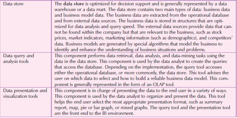
Figure 6.3(II) Basic BI Architectural components
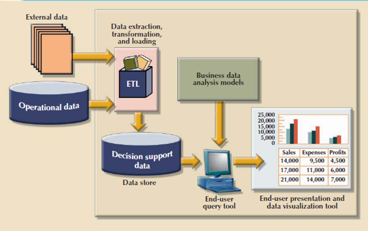
Figure 6.3(III) Business intelligence architectural components
Each BI component shown in has generated a fast-growing marketplace for specialized tools. And because of the advancement of client/server technologies, those components can interact with other components to make a very open architecture. As a matter of fact, you'll integrate multiple tools from different vendors into one BI framework.
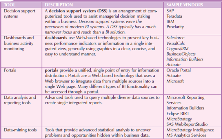

Figure 6.3(IV) Sample of Business intelligence tools
BI has a very important role in modern business operations, keep in mind that the manager must initiate the decision support process by asking the acceptable questions. The BI environment exists to support the manager; it doesn't replace the management function. If the manager fails to ask the appropriate questions, problems won't be identified and solved, and opportunities are going to be missed. In spite of the very powerful BI presence, the human component remains at the middle of business technology.
Although BI is used at strategic and tactical managerial levels within organizations, its effectiveness depends on the standard of data gathered at the operational level. Yet operational data are seldom compatible to the decision support tasks.
A. Operational Data vs. Decision Support Data
Operational data and decision support data having a different purposes. Therefore, it's not surprising to find out that their formats and structures differ. Most operational data are stored during a relational database during which the structures (tables) tend to be highly normalized.
Operational data storage is used to support transactions that represent daily operations. For instance, whenever an item is sold, it must be accounted for. Customer data, inventory data, and so on, are during a frequent update mode. To supply effective update performance, operational systems store data in many tables, each with a minimum number of fields. Thus, a simple sales transaction could be represented by five or more different tables. Although such an arrangement is superb in an operational database, it's not efficient for query processing. For instance, to extract a simple invoice, you'd need to join several tables.
Whereas operational data are useful for capturing daily business transactions, decision support data give tactical and strategic business to the operational data. From the data analyst’s point of view, decision support data different from operational data in three main areas: time span, granularity, and dimensionality.
Figure shows how decision support data are often examined from multiple dimensions using a type of filters to supply each dimension. The power to analyze, extract, and present information in meaningful ways is one among the differences between decision support data and transaction-at-a-time operational data.From the designer’s point of view, the differences between operational and decision support data are as follows:
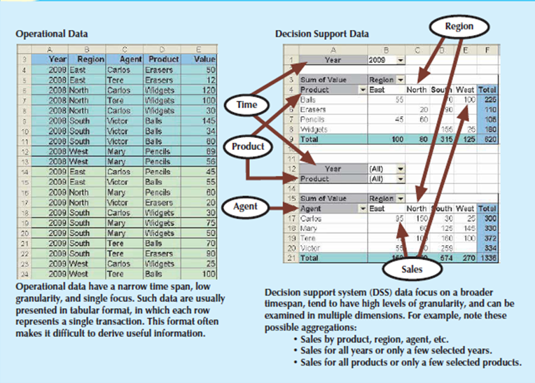
Figure 6.4(I) Transforming operational data into decision support data
Decision support data could be collected to observe such aggregates as total sales for every store or for every product. The purpose of the summaries is simple: they're to be used to establish and evaluate sales trends, product sales comparisons, and so on, that serve decision needs.
Therefore, decision support databases used to be non-normalized and include few tables, each of which contains a large number of attributes.
Table shows the differences between operational and decision support data from the database designer’s point of view.
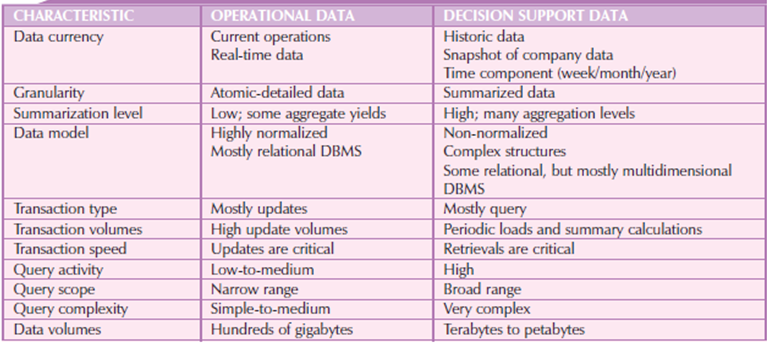
Figure 6.4(II) Contrasting Operational and Decision Support Data Characteristics
B. Decision Support Database Requirements
A decision support database may be a specialized DBMS tailored to supply fast answers to complex queries. There are four requirements for a decision support database that is the database schema, data extraction and loading, the end-user analytical interface, and database size.
Database Schema
The decision support database schema support complex data representations. The decision support database consist of data that are aggregated and summarized. Additionally to fulfill those requirements, the queries need to extract multidimensional time slices. If you're using an RDBMS, the conditions suggest using non-normalized and even duplicated data. To see why this must be true, take a look at the 10-year sales history for one store containing one department. At now, the info are fully normalized within the only table shown in figure.
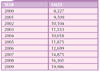
Figure 6.4(III) Ten-Year Sales History for a Single Department, in Millions of Dollars
Department, in Millions of Dollars
This structure works well once you have just one store with just one department. However, it's impossible that such a simple environment has much need for a choice support database. One would suppose that a decision support database becomes a factor when handling quite one store, each of which has more than one department.
To support all of the decision support requirements, the database must contain data for all of the stores and every one of their departments and therefore the database must be ready to support multidimensional queries that track sales by stores, by departments, and over time.
Consider that there are only two stores (A and B) and two departments (1 and 2) within each store. Let’s also change the time dimension to add yearly data. Following table shows the sales figures under the required conditions. Only 2000, 2004, and 2009 are shown; ellipses (...) are wont to indicate that data values were omitted.
Data Extraction and Filtering
The decision support database is made largely by extracting data from the operational database and by importing additional data from external sources. Therefore, the DBMS need to support advanced data extraction and data-filtering tools.
To overcome the impact on the operational database, the data extraction capabilities should allow batch and scheduled data extraction. The data extraction capabilities support different data sources: flat files and hierarchical, network, and relational databases and multiple vendors. Data-filtering capabilities include the ability to see for inconsistent data or data validation rules. Finally, to filter and integrate the operational data into the decision support database, the DBMS must support advanced data integration, aggregation, and classification.
Using data from multiple external sources also usually means having to solve data-formatting conflicts. For instance, data like Social Security numbers and dates can occur in several formats; measurements are often supported different scales, and therefore the same data elements can have different names.
End-User Analytical Interface
The decision support DBMS need to support advanced data-modeling and data presentation tools. Using these tools makes it easy for data analysts to define the nature and extent of business problems. Once the problems defined, the decision support DBMS generate the necessary queries to retrieve the appropriate data from the decision support database.
If required then the query results may evaluated with data analysis tools supported by the decision support DBMS. Because queries yield crucial information for decision makers, the queries need to optimize for speedy processing. The end-user analytical interface is most critical DBMS components. An analytical interface permits the user to navigate through the data to simplify and accelerate the decision-making process.
Database Size
Decision support databases is very large; gigabyte and terabyte ranges aren't unusual. For instance, in 2008, Wal-Mart, the world’s largest company, had quite 4 petabytes of data in its data warehouses. The decision support database contains redundant and duplicated data to enhance data retrieval and simplify information generation.
Therefore, the DBMS is capable of supporting very large databases (VLDBs). To support a VLDB, the DBMS could be required to use advanced hardware, like multiple disk arrays, and to support multiple-processor technologies, like a symmetric multiprocessor (SMP) or a massively parallel processor (MPP).
The complex information requirements and then the ever-growing demand for sophisticated data analysis sparked the creation of a new form of data repository. This repository contains data in formats that support data extraction, data analysis, and deciding. This data repository is understood as a data warehouse and has become the foundation for a new generation of decision support systems.
Bill Inmon, is the “father” of the data warehouse, defines the term as “an integrated, subject-oriented, time-variant, nonvolatile collection of data that gives support for decision making.” to know that definition consider the following components.
Although this requirement sounds logical, you'd be amazed to get what percentage different measurements for “sales performance” can exist within an organization; an equivalent scenario holds true for the other business element. as an example , the status of an order could be indicated with text labels like “open,” “received,” “canceled,” and “closed” in one department and as “1,” “2,” “3,” and “4” in another department.
A student’s status could be defined as “freshman,” “sophomore,” “junior,” or “senior” within the accounting department and as “FR,” “SO,” “JR,” or “SR” within the computer information systems department. To avoid the potential format tangle, the information within the data warehouse need to conform to a common format acceptable throughout the organization. This integration are often time-consuming, but once accomplished, it enhances deciding and helps managers better understand the company’s operations. These understandings are often translated into recognition of strategic business opportunities.
This type of data organization is sort of different from the more functional or process-oriented organization of typical transaction systems. For instance, an invoicing system designer focus on designing normalized data structures to support the business process by storing invoice components in two tables: INVOICE and INVLINE.
In contrast, the data warehouse features a subject orientation. Data warehouse designers focus specifically on the data instead of on the processes that modify the data. Therefore, rather than storing an invoice, the data warehouse stores its “sales by product” and “sales by customer” components because decision support activities need the retrieval of sales summaries by product or customer.
For instance, when data for previous weekly sales are uploaded to the data warehouse, the weekly, monthly, yearly, and other time-dependent aggregates for products, customers, stores, and other variables are also updated. Because data during a data warehouse with a snapshot of the company history as measured by its variables, the time component is crucial. The data warehouse contains a time ID which is used to generate summaries and aggregations by week, month, quarter, and year. Once the information enter the data warehouse, the time ID assigned to the information can't be changed.
That’s why the DBMS must be ready to support multi-gigabyte and even multi-terabyte or greater databases, operating on multiprocessor hardware. Table shows the differences between data warehouses and operational databases.
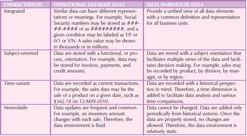
Figure 6.5(I)Characteristics of Data Warehouse Data and Operational Database Data
Typically, data are extracted from various sources and are then transformed and integrated in other words, skilled an information filter before being loaded into the data warehouse. As mentioned, this process of extracting, transforming, and loading the aggregated data into the data warehouse is understood as ETL. Following figure shows the ETL process to make a data warehouse from operational data.
Although the centralized and integrated data warehouse are attractive proposition that provides many benefits, managers could also be reluctant to embrace this strategy. Creating a data warehouse needs time, money, and considerable managerial effort. Therefore, it's not surprising that a lot of companies begin their foray into data warehousing by that specialize in more manageable data sets that are targeted to fulfill the special needs of small groups within the organization. These smaller data stores are called data marts.
A data mart may be a small, single-subject data warehouse subset that gives decision support to a little group of individuals. Additionally, a data mart could even be created from data extracted from a bigger data warehouse with the precise function to support faster data access to a target group or function. That is, data marts and data warehouses can coexist within a business intelligence environment.
Some organizations prefer to implement data marts not only due to the lower cost and shorter implementation time but also due to the current technological advances and inevitable “people issues” that make data marts attractive. Powerful computers can provide a customized decision support system to small groups in ways in which won't be possible with a centralized system. Also, a company’s culture predispose its employees to resist major changes, but they quickly embrace relatively minor changes that cause demonstrably improved decision support.
Additionally, people at different organizational levels are likely to need data with different summarization, aggregation, and presentation formats. Data marts used as a test vehicle for companies exploring the potential benefits of data warehouses. By gradually migrating from data marts to data warehouses, a selected department’s decision support needs are often addressed within an inexpensive time-frame as against the longer time-frame usually required to implement a data warehouse.
Information technology (IT) departments also benefit from this approach because their personnel have the chance to find out the problems and develop the talents required to make a data warehouse.
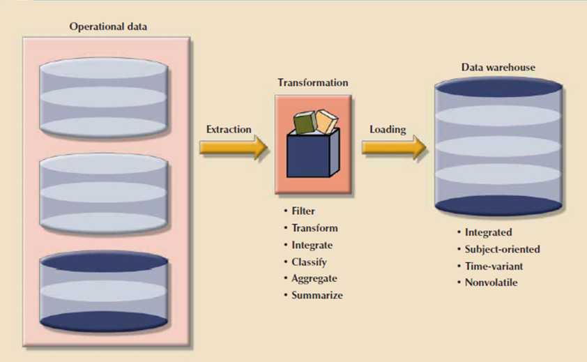
Figure 6.5(II) The process
The difference between a data mart and a data warehouse is the size and scope of the problem was solved.
Therefore, the problem definitions and data requirements are essentially an equivalent for both. The data warehouse must conform to uniform structures and formats to avoid data conflicts and to support decision making. In fact, before a decision support database are considered a true data warehouse.
A. Twelve Rules that define a data Warehouse
In 1994, William H. Inmon and Chuck Kelley created 12 rules defining a knowledge warehouse.
1. The data warehouse and operational environments are separated.
2. The data warehouse data are integrated.
3. The data warehouse contains historical data over an extended time.
4. The data warehouse data is snapshot data captured at a particular point in time.
5. The data warehouse data are subject oriented.
6. The data warehouse data is read-only with periodic batch updates from operational data. No online updates are allowed in this.
7. The data warehouse development life cycle different from classical systems development. The data warehouse development is data-driven and the classical approach is process-driven.
8. The data warehouse consist of data with several levels of details that is current detail data, old detail data, lightly summarized data, and highly summarized data.
9. The data warehouse environment is characterized by read-only transactions to very large data sets. The operational environment is characterized by numerous update transactions to a couple of data entities at a time.
10. The data warehouse environment features a system that traces data sources, transformations, and storage.
11. The data warehouse’s metadata are a critical component of this environment. The metadata identify and define all data elements. The metadata provide the source, transformation, integration, storage, usage, relationships, and history of every data element.
12. The data warehouse contains a chargeback process for resource usage that perform optimal use of the data by end users.
These 12 rules introduce entire data warehouse life cycle from its introduction as an entity break away the operational data store to its components, functionality, and management processes.
B. Decision Support Architectural Styles
Several decision support database architectural styles are available. These architectures provide advanced decision support features, and a few are capable of providing access to multidimensional data analysis. Following table shows the most architectural styles that you simply are likely to encounter within the decision support database environment.
An entire data warehouse architecture has support for a decision support data store, a data extraction and integration filter, and a specialized presentation interface.
The need for more intensive decision support prompted the introduction of latest generation of tools. Those new tools, called online analytical processing (OLAP), create a complicated data analysis environment that supports decision making, business modeling, and operations research. OLAP systems has four main characteristics:
Let’s examine each of these characteristics.
A. Multidimensional Data Analysis Techniques
The most important characteristic of recent OLAP tools is the capacity for multidimensional analysis. In multidimensional analysis the data are processed and viewed as a part of a multidimensional structure. This kind of data analysis is attractive to business decision makers because they have a tendency to look at business data as data that are associated with other business data.
To understand this view study how a business data analyst might investigate sales figures. During this, the analyst is curious about the sales figures as they relate to other business variables like customers and time. In other words, customers and time are viewed as different dimensions of sales. Figure shows how the operational view differs from the multidimensional view of sales.
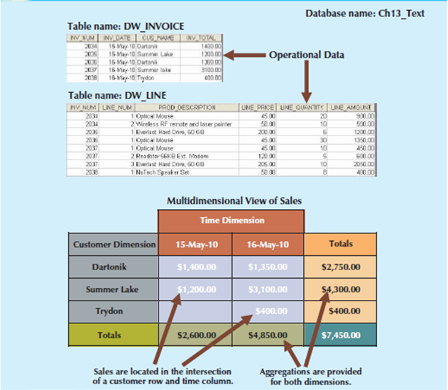
Figure 6.6 (I)Operational vs. multidimensional view of sales
As shown in figure the tabular (operational) view of sales data isn't compatible to decision support, because the relationship between INVOICE and LINE doesn't provide a business perspective of the sales data. On the opposite hand, the end user’s view of sales data from a business perspective is more closely represented by the multidimensional view of sales than by the tabular view of separate tables.
The multidimensional view support end users to consolidate or aggregate data at different levels: total sales figures by customers and by date. Finally, the multidimensional view of data allows a business data analyst to simply switch business perspectives from sales by customer to sales by division, by region, and so on. Multidimensional data analysis techniques are augmented by the subsequent functions:
• Advanced data presentation functions. 3-D graphics, pivot tables, crosstabs, data rotation, and 3 dimensional cubes. These facilities are compatible with desktop spreadsheets, statistical packages, and query and report packages.
• Advanced data aggregation, consolidation, and classification functions. These allow the data analyst to make multiple data aggregation levels, slice and dice data, and drill down and roll up data across different dimensions and aggregation levels. For instance, aggregating data across the time dimension like week, month, quarter, and year which allows the data analyst to drill down and roll up across time dimensions.
• Advanced computational functions. These contains business-oriented variables, financial and accounting ratios, and statistical and forecasting functions. These functions are provided automatically, and therefore the user doesn't have to redefine their components when they're accessed.
• Advanced data-modeling functions. These provide support for what-if scenarios, variable assessment, and variable contributions to outcome, linear programming, and other modeling tools.
Because many analysis and presentation functions are common to desktop spreadsheet packages, most OLAP vendors have closely integrated their systems with spreadsheets like Microsoft Excel. Using the features available in graphical end-user interfaces like Windows, the OLAP menu option simply becomes an alternative choice within the spreadsheet menu bar.
This seamless integration is a plus for OLAP systems and for spreadsheet vendors because end users gain access to advanced data analysis features by using familiar programs and interfaces. Therefore, additional training and development costs was reduced.
B. Advanced Database Support
To provide efficient decision support, OLAP tools have advanced data access features. Which includes:
• Access to several different sorts of DBMSs, flat files, and internal and external data sources.
• Access to aggregated data warehouse data also on the detail data found in operational databases.
• Advanced data navigation features like drill-down and roll-up.
• Rapid and consistent query response times.
• The ability to map end-user requests, expressed in either business or model terms, to the acceptable data source then to the right data access language. The query code must be optimized to match the info source, no matter whether the source is operational or data warehouse data.
• Support for very large databases. The data warehouse easily and quickly grow to multiple gigabytes and even terabytes.
To provide a seamless interface, OLAP tools map the data elements to the data warehouse and from the operational database to their own data dictionaries. These metadata are used to translate end-user data analysis requests into the right query codes, which are then directed to the acceptable data source.
C. Easy-to-Use End-User Interface
Advanced OLAP features is more useful when access to them is very simple. OLAP tool vendors learned this concept early and equipped their sophisticated data extraction and analysis tools with easy-to-use graphical interfaces. Multiple interface features are “borrowed” from previous generations of data analysis tools which are familiar to finish users. This familiarity makes OLAP easily accepted and readily used.
D. Client/Server Architecture
Client/server architecture provides a framework within which new systems are often designed, developed, and implemented. The client/server environment enables an OLAP system to be divided into several components that outline its architecture. Those components can then be placed on an equivalent computer, or they will be distributed among several computers. Thus, OLAP is meant to satisfy ease-of-use requirements while keeping the system flexible.
E. OLAP Architecture
OLAP operational characteristics are often divided into three main modules:
In the client/server environment these three OLAP modules make the features of OLAP such as multidimensional data analysis, advanced database support, and an easy-to-use interface. Following figure shows OLAP’s client/server components and attributes.
As Figure shows OLAP systems are designed to use both operational and data warehouse data. The OLAP system components located on one computer, but this single-user scenario is merely one among many. There is a one problem with the installation shown here is that every data analyst must have a strong computer to store the OLAP system and perform all processing locally. Additionally, each analyst uses a separate copy of the data.
Therefore, the data copies must be synchronized to make sure that analysts are working with an equivalent data. In other words, each user must have his/her own “private” copy of the data and programs. This approach doesn't provide the advantages of one business image shared among all users.
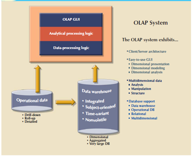
figure 6.6 (II) OLAP client/server architecture
A more common architecture is one during which the OLAP GUI runs on client workstations and the OLAP engine, or server, composed of the OLAP analytical processing logic and OLAP data-processing logic which is runs on a shared computer. In this OLAP server are going to be a front end to the data warehouse’s decision support data.
This front end or middle layer accepts and processes the data-processing requests formed by the multiple end-user analytical tools. The end-user GUI could be a custom-made program or a plug-in module that's integrated with spreadsheet software or a third-party data analysis and query tool.
The data warehouse is traditionally created and maintained by a process or software tool that's independent of the OLAP system. This independent software performs the data extraction, filtering, and integration used to transform operational data into data warehouse data. This scenario reflects the fact that the data warehousing and data analysis activities are handled separately.
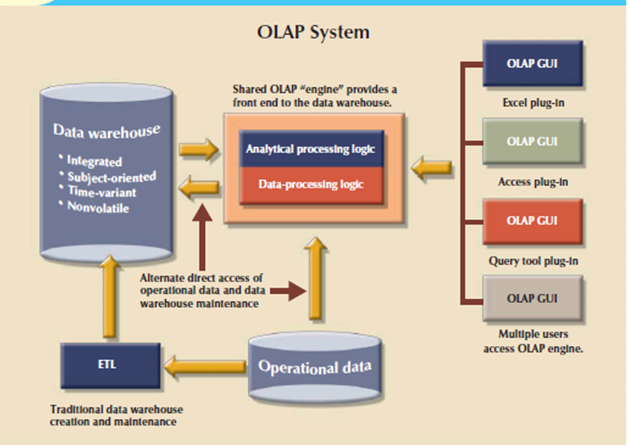
Figure 6.6(III) OLAP server arrangement
At now, you would possibly ask why you would like a data warehouse if OLAP provides the required multidimensional data analysis of operational data. the solution lies within the definition of OLAP. OLAP is defined as “advanced data analysis environment which supports decision making, business modeling, and research activities.” The keyword present is environment, which incorporates client/server technology.
Environment is defined as “surroundings or atmosphere.” And an environment surrounds a nucleus. During this case, the nucleus consists of all business activities within an organization as represented by the operational data.
Even as there are several layers within the atmosphere, there are several layers of knowledge processing, with each outer layer representing a more aggregated data analysis. the very fact is that an OLAP system might access both data storage types or only one; it depends on the vendor’s implementation of the product selected. In any case, multidimensional data analysis requires some kind of multidimensional data representation, which is generally provided by the OLAP engine.
In various implementations, the data warehouse and OLAP are interrelated, complementary environments. And the data warehouse holds integrated, subject-oriented, time-variant, and nonvolatile decision support data, the OLAP system provides the front end through which end users access and analyze such data.
OLAP system directly access operational data, transforming it and storing it during a multidimensional structure. That means the OLAP system can provide an alternate multidimensional data store component, as shown in Figure.
Figure describe a scenario during which the OLAP engine extracts data from an operational database then stores it during a multidimensional structure for further data analysis. The extraction process follows an equivalent conventions used with data warehouses.
Therefore, the OLAP provides a mini data-warehouse component that appears remarkably just like the data mart mentioned in previous sections. During this scenario, the OLAP engine perform all of the data extraction, filtering, integration, classification, and aggregation functions which data warehouse provides.
In fact, when properly implemented, the data warehouse performs all data preparation functions rather than letting OLAP perform, those chores; as a result, there's no duplication of functions. Better yet, the info warehouse handles the data component more efficiently than OLAP does, so you'll appreciate the advantages of getting a central data warehouse serve as the large enterprise decision support database.
To provide high performance the OLAP systems merge the data warehouse and data mart approaches by storing small extracts of the data warehouse at end-user workstations. The objective is to extend the speed of data access and data visualization. The logic of using this approach is that the assumption that the majority end users work with fairly small, stable data warehouse data subsets. For instance, a sales analyst is work with sales data, and a customer representative is likely to work with customer data. Following figure illustrates that scenario.
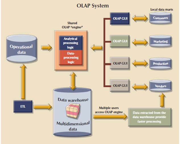
Figure 6.6 (IV) OLAP server with local mini-data-marts
In arrangement of the OLAP components, one thing is important that multidimensional data must be used. But how are multidimensional data is stored and managed? OLAP proponents are sharply divided. Some favor the use of relational databases to store the multidimensional data; others argue for the prevalence of specialized multidimensional databases for storing multidimensional data. The essential characteristics of every approach are examined next.
F. Relational OLAP
Relational online analytical processing (ROLAP) provides OLAP functionality by using relational databases and relational query tools used to store and analyze multidimensional data.
That approach builds on existing relational technologies and represents a natural extension to all or any of the companies that already use relational database management systems within their organizations. ROLAP adds the subsequent extensions to traditional RDBMS technology:
Multidimensional Data Schema Support within the RDBMS
Relational technology uses normalized tables to store data. The reliance on normalization because the design methodology for relational databases is consider as obstacle to its use in OLAP systems. Normalization divides business entities into smaller pieces to supply the normalized tables. For instance, sales data components could be stored in four or five different tables.
The reason for using normalized tables is to overcome redundancies, eliminating data anomalies, and facilitate the data updates. For decision support purposes, it's easier to know data once they are seen with reference to other data. As long view of the data environment decision support data used as non-normalized, duplicated, and pre-aggregated. Those characteristics seem to make impossible the use of standard relational design techniques and RDBMSs because the foundation for multidimensional data.
Those who heavily invested in relational technology, ROLAP uses a special design technique to enable RDBMS technology to support multidimensional data representations. This special design technique is known as a star schema.
The star schema is meant to optimize data query operations instead of data update operations. Changing the data design foundation means the tools are access such data will need to change. End users who are familiar with the traditional relational query tools will discover that those tools don't work efficiently with the new star schema. Therefore ROLAP saves the day by adding support for the star schema when know query tools are used. ROLAP provides advanced data analysis functions and improves query optimization and data visualization methods.
Data Access Language and Query Performance Optimized for Multidimensional Data
Another criticism of relational databases is that SQL isn't suitable to performing advanced data analysis. Most decision support data requests needs the use of multiple-pass SQL queries or multiple-nested SQL statements. To answer this criticism, ROLAP extends SQL in way that it can differentiate between access requirements for data warehouse data and operational data. Therein way, a ROLAP system is able to get the SQL code required to access the star schema data.
Query performance is additionally improved because the query optimizer is modified to identify the SQL code’s intended query targets. For instance, if the query target is that the data warehouse, the optimizer passes the requests to the data warehouse.
If the end user performs drill-down queries against operational data, the query optimizer identifies that operation and optimizes the SQL requests before passing them to the operational DBMS.
Another way of improved query performance is the use of advanced indexing techniques such as bitmapped indexes within relational databases. Because the name suggests, a bitmapped index is predicated on 0 and 1 bits to represent a given condition. For instance , if the REGION attribute in has only four outcomes North, South, East, and West those outcomes could also be represented as shown in Table. The “1” represents “bit on,” and therefore the “0” represents “bit off.” for instance , to represent a row with a region attribute = “East,” only the “East” bit would get on .
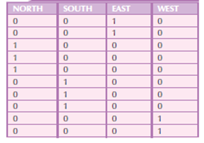
Figure 6.6(V) Bitmap Representation of Region Values
The index in above Table takes a minimum amount of space. The bitmapped indexes are efficient at handling large amounts of data than indexes present in many relational databases. But do assumed that bitmapped indexes are primarily used in situations where the number of possible values for an attribute is fairly small. For instance, REGION has only four outcomes during this example.
Marital status married, single, widowed, divorced is another good bitmapped index candidate, as gender M or F. ROLAP tools are mainly client/server products during which the end-user interface, the analytical processing, and therefore the data processing happen on different computers. Following figure shows the interaction of the client/server ROLAP components.
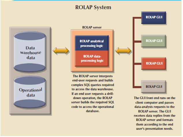
Figure 6.6(VI) Typical ROLAP client/server architecture
Support for Very Large Databases
Recall that support for VLDBs may be a requirement for decision support databases. Therefore, when the relational database is used during a decision support role, it also must be ready to store very large amounts of data. Both the storage capability and therefore the process of loading data into the database are crucial. Therefore, the RDBMS must have the proper tools to import, integrate, and populate the data warehouse with data.
Decision support data are normally loaded in bulk (batch) mode from the operational data. However, batch operations require that both the source and therefore the destination databases be reserved (locked). The speed of the data-loading operations is vital, especially once you realize that the majority operational systems run 24 hours each day, 7 days every week, 52 weeks a year. Therefore, the window of opportunity for maintenance and batch loading is open only briefly, typically during slack periods.
With an open client/server architecture, ROLAP provides advanced decision support capabilities that are scalable to the whole enterprise. Clearly, ROLAP may be a logical choice for companies that already use relational databases for his or her operational data. Given the size of the relational database market, it's hardly surprising that the majority current RDBMS vendors have extended their products to support data warehouses.
G. Multidimensional OLAP
Multidimensional online analytical processing means MOLAP extends OLAP functions to multidimensional database management systems that is MDBMSs. MOLAP’s premise is that multidimensional databases are suited to manage, store, and analyze multidimensional data. Many proprietary techniques utilized in MDBMSs are from engineering fields such as computer-aided design/computer-aided manufacturing (CAD/CAM) and geographic information systems (GIS).
MDBMS end users visualize the stored data as a 3 dimensional cube as a data cube. The location of every data value within the data cube is a function of the x-, y-, and z-axes during a three-dimensional space. The x-, y-, and z-axes shows the dimensions of the data value. The data cubes can grow to n number of dimensions, thus becoming hypercube.
Data cubes are created by extracting data from the operational databases or data warehouse. One important characteristic of data cubes is that they're static; that’s, they're not subject to vary and must be created before they will be used. Data cubes can't be created by ad hoc queries. Instead of you use query pre-created cubes with defined axes. For instance, a cube for sales contains the product, location, and time dimensions, and you'll query only those dimensions. Therefore, the data cube creation process is critical and needs in-depth front-end design work.
The front-end design work could also be well justified because MOLAP databases are known to be much faster than their ROLAP counterparts, especially when handling small-to-medium-sized data sets. To speed data access, data cubes are present in memory in what's called the cube cache. Because MOLAP benefits from a client/server infrastructure, the cube cache are located at the MOLAP server, at the MOLAP client, or in both locations. Following figure shows the essential MOLAP architecture.
Because the data cube is predefined with a set number of dimensions, the addition of a new dimension needs the whole data cube be re-created. This re-creation process is time-consuming. Therefore, when data cubes are created too often, the MDBMS loses a number of its speed advantage over the relational database. And although MDBMSs have performance advantages over relational databases, the MDBMS is best suited to small and medium-sized data sets.
Scalability is somewhat limited because the size of the data cube is restricted to avoid lengthy data access times caused by having less work space available for the OS and therefore the application programs. Additionally, the MDBMS makes use of proprietary data storage techniques that require proprietary data access methods using a multidimensional query language.
Multidimensional data analysis is affected by how the database system handles sparsity. Sparsity is a measurement of the density of the data within the data cube and is computed by dividing the total number of actual values within the cube by the total number of cells within the cube. Because the data cube’s dimensions are predefined, not all cells are populated.
In other words, some cells are empty. Returning to the sales example, there could also be many products that aren't sold during a given period of time during a given location. In fact, you'll often find that fewer than 50 percent of the info cube’s cells are populated. In any case, multidimensional databases need to handle sparsity to reduce processing overhead and resource requirements.
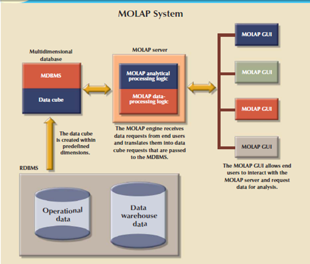
Figure 6.6(VII) MOLAP client/server architecture
Relational proponents argue that using proprietary solutions makes it difficult to integrate the MDBMS with other data sources and tools used within the enterprise. Although it takes a considerable investment of your time and effort to integrate the new technology and therefore the existing information systems architecture, MOLAP could also be a good solution for those situations during which small-to-medium-sized databases are the norm and application software speed is critical.
H. Relational vs. Multidimensional OLAP
Table shows some OLAP and MOLAP pros and cons. keep in mind, too, that the selection of 1 or the other often depends on the evaluator’s viewpoint. For instance, a correct evaluation of OLAP must include price, supported hardware platforms, compatibility with the existing DBMS, programming requirements, performance, and availability of administrative tools.
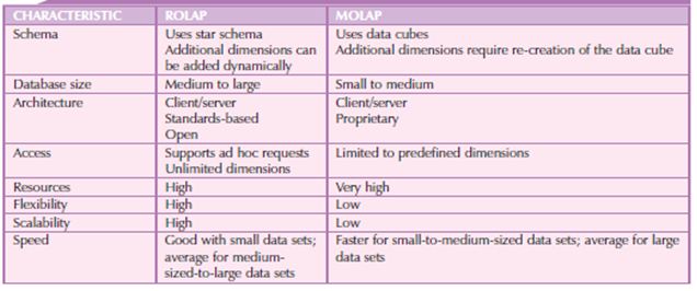
Figure 6.6(VIII) Relational vs. Multidimensional OLAP
ROLAP and MOLAP vendors are working with the mixing of their respective solutions within a unified decision support framework. Many OLAP products are ready to handle tabular and multidimensional data with an equivalent ease.
For example, if you're using Excel OLAP functionality, you'll access relational OLAP data during a SQL server also as cube data within the local computer. Within the meantime, relational databases successfully use the star schema design to handle multidimensional data, and their market share makes it unlikely that their popularity will fade anytime soon.
The star schema may be a data-modeling technique won’t to map multidimensional decision support data into a relational database. The star schema creates the same as a multidimensional database schema from the existing relational database. The star schema developed because existing relational modeling techniques, ER, and normalization not provide a database structure that fulfill advanced data analysis requirements well.
Star schemas is easily implemented model for multidimensional data analysis while still preserving the relational structures on which the operational database is made. The star schema consist of four components such as facts, dimensions, attributes, and attribute hierarchies.
A. Facts
Facts are numeric measurements that describes a selected business aspect or activity. For instance, sales figures are numeric measurements that show product and service sales. Facts are used in business data analysis are units, costs, prices, and revenues. Facts are stored during a fact table that's the middle of the star schema. The fact table contains facts which are linked through their dimensions.
Facts are computed or derived at run time. These computed or derived types of facts are called metrics to differentiate them from stored facts. The fact table is updated periodically with data from operational databases.
B. Dimensions
Dimensions are qualifying characteristics that provide additional perspectives to a given fact. Dimensions are of interest because decision support data are always viewed in relation to other data. As an example, sales was compared by product from region to region and from one time period to subsequent.
The type of problem addressed by a BI system to form a comparison of the sales of unit X by region for the primary quarters of 2000 through 2010. Therein example, sales have product, location, and time dimensions. In effect, dimensions are the magnifying glass through which you study the facts. Such dimensions are normally stored in dimension tables.
Figure shows a star schema for sales with product, location, and time dimensions.
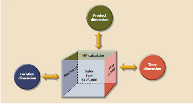
Figure 6.7(I) Simple star schema
C. Attributes
Each dimension table contains attributes. Attributes are used to search, filter, or classify facts. Dimensions provide descriptive characteristics about the facts through their attributes. Then the data warehouse designer need to define common business attributes which was employed by the data analyst to narrow an enquiry, group information, or describe dimensions. Using a sales example, some possible attributes for every dimension are shown in Table.


Figure 6.7(II) Possible Attributes for Sales Dimensions
These product, location, and time dimensions add a business perspective to the sales facts. The data analyst group the sales figures for a given product, during a given region, and at a given time. The star schema, through its facts and dimensions, can provide the info within the required format when the data are needed. And it can do so without imposing the burden of the extra and unnecessary data that commonly exist in operational databases.
The sales example’s multidimensional data model is suitable to represent by a three-dimensional cube. Of course, this doesn't imply that there's a limit on the number of dimensions which will be associated to a fact table.
There is no mathematical limit to the number of dimensions used. But using a three-dimensional model makes it easy to see the problem. During this three-dimensional example, the multidimensional data analysis terminology, the cube shown in Figure represents a view of sales dimensioned by product, location, and time.
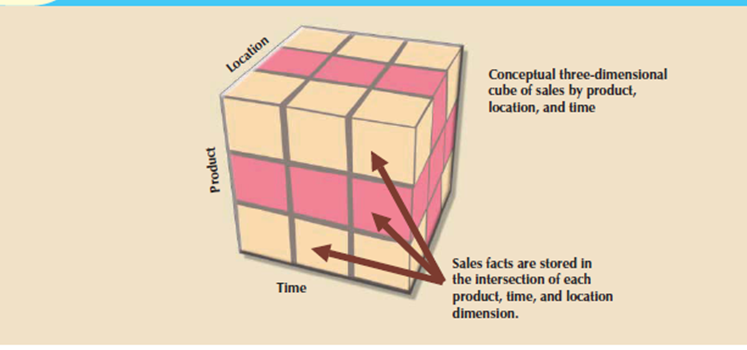
Figure 6.7(III) Three-dimensional view of sales
Every sales value stored within the cube is related to the location, product, and time dimensions. However, this cube is simply a conceptual representation of multidimensional data, and it doesn't show how the information is physically stored during a data warehouse.
A ROLAP engine stores data in an RDBMS and uses its own data analysis logic and then the end-user GUI to perform multidimensional analysis. A MOLAP system stores data in an MDBMS with the help of proprietary matrix and array technology to simulate this multidimensional cube.Whatever the underlying database technology the main features of multidimensional analysis is its ability to concentrate on specific “slices” of the cube.
For example, the product manager curious about examining the sales of a product while the shop manager is curious about examining the sales made by a specific store. In multidimensional terms, the ability to specialize in slices of the cube to perform a more detailed analysis is understood as slice and dice.
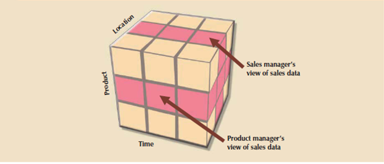
Figure 67(IV) Slice-and-dice view of sales
To slice and dice with the help of this it is possible to identify each slice of the cube. Which is done by using the values of every attribute during a given dimension. For instance, to use the situation dimension, you would possibly got to define a STORE_ID attribute so as to specialize in a specific store.
In above table consider that every attribute adds a further perspective to the sales facts, therefore setting the stage for locating new ways to look, classify, and possibly aggregate information.
For instance, the location dimension adds a geographic perspective of where the sales took place in which region, state, city, store, and so on. All of the attributes are selected with the target of providing decision support data to the end users in order that they will study sales by each of the dimension’s attributes.
Time is an important dimension. The time dimension provides a framework from which sales patterns are often analyzed and possibly predicted. The time dimension plays an important role when the data analyst is curious about looking at sales aggregates by quarter, month, week, and so on.
Given the importance and universality of the time dimension from a data analysis way in that many vendors added automatic time dimension management features to their data-warehousing products.
D. Attribute Hierarchies
Attributes within dimensions are often ordered during a well-defined attribute hierarchy. The attribute hierarchy provides a top-down data organization which is used for 2 main purposes that is aggregation and drill-down/roll-up data analysis. For instance, following figure shows how the location dimension attributes are often organized during a hierarchy by region, state, city, and store.
The attribute hierarchy provides the potential to perform drill-down and roll-up searches during a data warehouse. For instance, consider that a data analyst looks at the answers to the query: How does the 2009 month-to-date sales performance compare to the 2010 month-to-date sales performance? The data analyst point out a sharp sales decline for March 2010.
The data analyst might plan to drill down inside the month of March to check how sales by regions compared to the previous year. By doing that, the analyst can determine whether the low March sales were reflected altogether regions or in just a specific region. This sort of drill-down operation can even be extended until the data analyst identifies the shop that's performing below the norm.
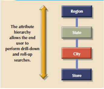
Figure 6.7(V) Location attribute hierarchy
The March sales scenario is feasible because the attribute hierarchy allows the data warehouse and OLAP systems to have a defined path which will identify how data are to be decomposed and aggregated for drill-down and roll-up operations. It’s not need for all attributes to be a part of an attribute hierarchy in that some attributes exist to supply narrative descriptions of the dimensions.
But understand that the attributes from different dimensions are grouped to make a hierarchy. For instance, after you drill down from city to store, you would possibly want to drill down using the product dimension in order that the manager can identify slow products within the store. The product dimension are often supported the product group (dairy, meat, then on) or on the product brand (Brand A, Brand B, then on).
Following figure illustrates a scenario during which the data analyst studies sales facts, using the product, time, and location dimensions. During this example, the product dimension is to “All products,” means that the data analyst will see all products on the y-axis.
The time dimension (x-axis) is “Quarter,” meaning that the data are aggregated by quarters. Finally, the location dimension is set to “Region,” thus ensuring that every cell contains the entire regional sales for a given product during a given quarter.
It provides the data analyst with three different information paths. On the product dimension (the y-axis), the data analyst can request to examine all products, products grouped by type, or simply one product. On the time dimension (the x-axis), the data analyst request time-variant data at different levels of aggregation such as year, quarter, month, or week.
Each sales value initially shows the entire sales, by region, of every product. When a GUI is used, clicking on the region cell enables the data analyst to drill right down to see sales by states within the region. Clicking again on one among the state values yields the sales for every city within the state, then forth.
As the preceding examples illustrate, attribute hierarchies determine how the data within the data warehouse are extracted and presented. The attribute hierarchy information is stored within the DBMS’s data dictionary and is used by the OLAP tool to access the info warehouse properly. Once such access is ensured, query tools must be closely integrated with the data warehouse’s metadata and that they must support powerful analytical capabilities.
E. Star Schema Representation
Facts and dimensions are normally represented by physical tables within the data warehouse database. The very fact table is said to every dimension table during a many-to-one (M:1) relationship. In other words, many fact rows are associated with each dimension row. Using the sales example, you'll conclude that every product appears repeatedly within the SALES fact table.
Fact and dimension tables are connected by foreign keys and are subject to the primary key/foreign key constraints. The primary key on the “1” side, the dimension table, is stored as a part of the primary key on the “many” side, the fact table. Because the fact table is related to several dimension tables, the primary key of the fact table may be a composite primary key.
Following figure show the relationships in the sales fact table and the product, location, and time dimension tables. To point out you ways easily the star schema are often expanded, a customer dimension has been added to the combination. Adding the customer dimension required including the CUST_ID within the SALES fact table and adding the CUSTOMER table to the database.
The composite primary key for the SALES fact table consists of TIME_ID, LOC_ID, CUST_ID, and PROD_ID.
Each record within the SALES fact table is uniquely identified by the mixture of values for every of the fact table’s foreign keys. By default, the fact table’s primary key's always formed by combining the foreign keys pointing to the dimension tables to which they're related. During this case, each sales record represents each product sold to a selected customer, at a selected time, and during a specific location.
During this schema, the TIME dimension table represents daily periods and the SALES fact table represents daily sales aggregates by product and by customer. Because fact tables contain the actual values used in the decision support process, those values are repeated repeatedly within the fact tables.
Therefore, the fact tables are always the most important tables within the star schema. Because the dimension tables contain only non-repetitive information, the dimension tables are always smaller than the fact tables.
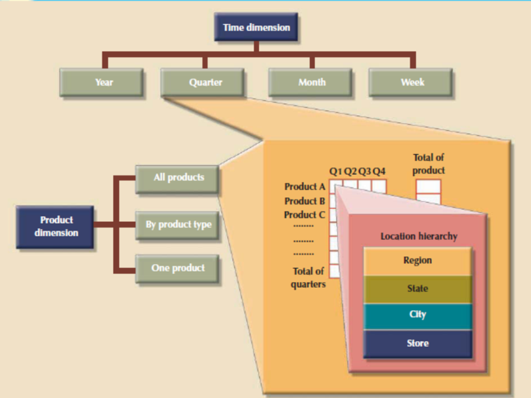
Figure 6.7(VI) Attribute hierarchies in multidimensional analysis
In a typical star schema, each dimension record is said to thousands of fact records. For instance, “widget” appears just one occasion within the product dimension, but it's thousands of corresponding records within the SALES fact table.
That characteristic of the star schema facilitates data retrieval functions because most of the time the data analyst will check out the facts through the dimension’s attributes. Therefore, a data warehouse DBMS that's optimized for decision support first searches the smaller dimension tables before accessing the larger fact tables.
Data warehouses contains many fact tables. Each fact table is meant to answer specific decision support questions. For instance, suppose that you simply develop a new interest in orders while maintaining your original interest in sales. Therein scenario, you should maintain an ORDERS fact table and a SALES fact table within the same data warehouse.
If orders are considered to be an organization’s key interest, the ORDERS fact table should be the center of a star schema which may have vendor, product, and time dimensions. Therein case, an interest in vendors yields a new vendor dimension, represented by a replacement VENDOR table within the database.
The product dimension is represented by an equivalent product table utilized in the initial sales star schema. However, given the interest in orders also as sales, the time dimension now requires special attention. If the orders department uses an equivalent time periods because the sales department, time are represented by the same schedule.
If different time periods are used when you want to create another table, named as ORDER_TIME need to represent the time periods used by the orders department. In following figure the orders star schema shares the product, vendor, and time dimensions.
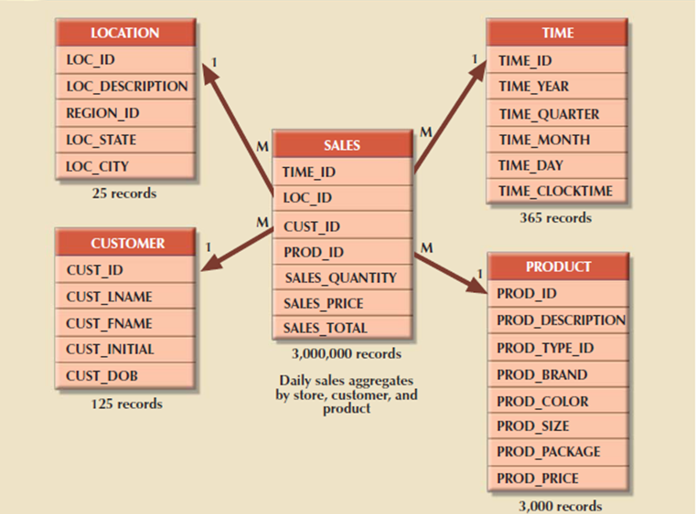
Figure 6.7(VII) Star schema for SALES
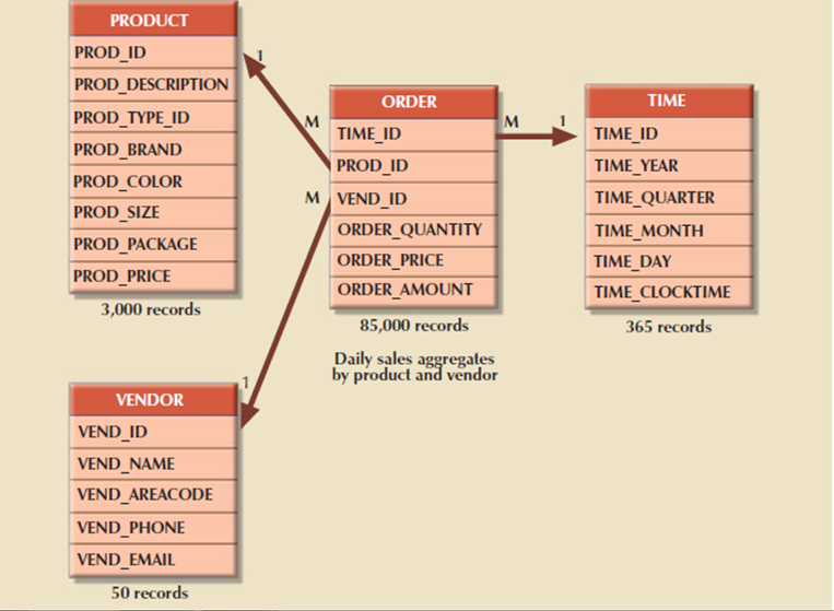
Figure 6.7(VIII) Orders star schema 13.7.6
F. Performance-Improving Techniques for the Star Schema
The creation of a database that gives fast and accurate answers to data analysis queries is that the data warehouse design’s prime objective. The performance-enhancement actions may target query speed through the use of SQL code also as through better semantic representation of business dimensions. These four techniques are used to create data warehouse design:
• Normalizing dimensional tables.
• Maintaining multiple fact tables to show different aggregation levels.
• De-normalizing fact tables.
• Partitioning and replicating tables.
Normalizing Dimensional Tables
Dimensional tables are normalized to get semantic simplicity and provide end-user navigation through the dimensions. For instance, if the location dimension table contains transitive dependencies within region, state, and city. The star schema is treated as a snowflake schema, which is a form of star schema during which the dimension tables can have their own dimension tables. The snowflake schema is the results of normalizing dimension tables.
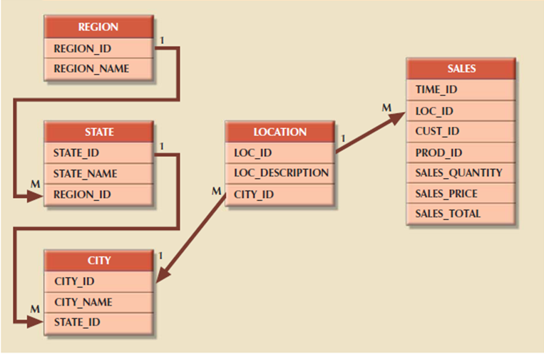
Figure 6.7(IX) Normalized dimension tables
By normalizing the dimension tables, you simplify the data-filtering operations related with the dimensions. During this example, the region, state, city, and location contain only a few records compared to the SALES fact table. Only the location table is directly related to the sales fact table.
Maintaining More Fact Tables to represent multiple Aggregation Levels
You can also speed up query operations by creating and maintaining multiple fact tables associated with each level of aggregation within the location dimension. These aggregate tables are pre-computed at the data-loading phase instead of at run time. The aim of this technique is to save many processor cycles at run time for speeding up data analysis.
An end-user query tool used for decision analysis then properly accesses the summarized fact tables rather than computing the values by accessing a lower level of detail fact table. This technique is shown in following Figure, which adds aggregate fact tables for region, state, and city to the initial sales example.
The data warehouse designer need to identify which levels of aggregation to pre-compute and store within the database. These many aggregate fact tables are updated in each load cycle in batch mode. Therefore the target is to minimize access and processing time, consistent with the expected frequency of use and therefore the processing time required to calculate a given aggregation level at run time, the data warehouse designer must select which aggregation fact tables to make .
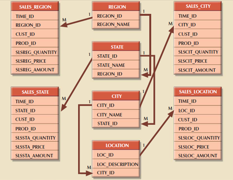
Figure 6.7(X) Multiple fact tables
Denormalizing Fact Tables
Denormalizing fact tables boost data access performance and saves data space for storing. The objective is to becoming less of a problem. Data storage costs decrease daily, and DBMS limitations which restrict database and table size limits, record size limits, and therefore the maximum number of records during a single table have much more negative effects than raw space for storing costs.
Denormalization improves performance by using a single record to store data that take many records. For instance, to compute the entire sales for all products altogether regions, you need to access the region sales aggregates and summarize all of the records during this table. If you've got 300,000 product sales, you'll be summarizing a minimum of 300,000 rows.
Although this not be taxing operation for a DBMS, a comparison of, say, 10 years’ worth of previous sales begins to bog down the system. In such cases, it's useful to have special aggregate tables that are denormalized. For instance, a YEAR_TOTALS table contain the subsequent fields: YEAR_ID, MONTH_1, MONTH_2 ... MONTH_12, and every year’s total. Such tables can easily be used to function a basis for year-to-year comparisons at the highest month level, the quarter level, or the year level.
Partitioning and Replicating Tables
Table partitioning and replication are important when a BI system is implemented in dispersed geographic areas. It is used to splits a table into subsets of rows or columns and places the subsets near to the client computer to increase data access time. Replication makes a replica of a table and places it during a different location, also to enhance access time.
No matter which performance-enhancement scheme is used, time is that the most common dimension utilized in business data analysis. Therefore, it's quite common to have one fact table for every level of aggregation defined within the time dimension.
For instance, within the sales example, you would possibly have five aggregate sales fact tables: daily, weekly, monthly, quarterly, and yearly. Those fact tables have an implicit or explicit periodicity defined. Periodicity consider as current year only, previous years, or all years, provides information about the time span of the info stored within the table.
At the end of every year, daily sales for the present year are moved to a different table that contains previous years’ daily sales only. This table contains all sales records from the start of operations, with the exception of the current year. The data within the current year and previous years’ tables represent the entire sales history of the company.
The previous year’s sales table are replicated at several locations to avoid having to remotely access the historic sales data, which may cause a slow response time. The possible size of this table is sufficient to intimidate about the bravest of query optimizers.
Organization-wide information system development is subject to several constraints. A number of the constraints are supported available funding. Others are a function of management’s view of the role played by an IS department and of the extent and depth of the data requirements. Add the constraints imposed by corporate culture, and you understand why no single formula can describe perfect data warehouse development.
Therefore, instead of proposing one data warehouse design and implementation methodology, this section identifies a couple of factors that appear to be common to data warehousing.
A. The Data Warehouse as an active Decision Support Framework
Perhaps the primary thing to recollect is that a data warehouse isn't a static database. Instead, it's a dynamic framework for decision support that’s, almost by definition, always a work in progress. Because it's the foundation of a modern BI environment, the design and implementation of the data warehouse means you're involved within the design and implementation of a complete database system development infrastructure for company-wide decision support.
Although it's easy to focus on the data warehouse database because the BI central data repository, you must remember that the decision support infrastructure includes hardware, software, people, and procedures, also as data. The argument that the info warehouse is that the only critical BI success component is as misleading because the argument that a person's being needs only a heart or a brain to function.
The data warehouse may be a critical component of a modern BI environment, but it's never the only critical component. Therefore, its design and implementation must be examined in light of the whole infrastructure.
B. A Company-Wide Effort that needs User Involvement
Designing a data warehouse means being given a chance to assist develop an integrated data model that captures the information that are considered to be essential to the organization, from both end-user and business perspectives. Data warehouse data cross departmental lines and geographical boundaries.
Because the data warehouse represents an effort to model all of the organization’s data, you're likely to get that organizational components often have conflicting goals, and it certainly are going to be easy to find data inconsistencies and damaging redundancies. Information is power, and therefore the control of its sources and uses is probably going to trigger turf battles, end-user resistance, and power struggles in the least levels.
Building the perfect data warehouse isn't just a matter of knowing the way to create a star schema; it requires managerial skills to affect conflict resolution, mediation, and arbitration. In short, the designer must:
• Involve end users within the process.
• Secure end users’ commitment from the start .
• Solicit continuous end-user feedback.
• Manage end-user expectations.
• Establish procedures for conflict resolution.
C. Satisfy the Trilogy: Data, Analysis, and Users
Great managerial skills aren’t, of course, solely sufficient. The technical aspects of the data warehouse must be addressed also. The old adage of input-process-output repeats itself here. The data warehouse designer must satisfy:
• Data integration and loading criteria.
• Data analysis capabilities with acceptable query performance.
• End-user data analysis needs.
The foremost technical concern in implementing a data warehouse is to supply end-user decision support with advanced data analysis capabilities—at the proper moment, within the right format, with the proper data, and at the proper cost.
Apply Database Design Procedures
The traditional database design procedures must adapted to suit the data warehouse requirements. If you remember that the data warehouse derives its data from operational databases, you'll understand why a solid foundation in operational database design is vital. Figure shows a simplified process for implementing the info warehouse.
As noted, developing a data warehouse may be a company-wide effort that needs many resources: human, financial, and technical. Providing company-wide decision support requires a sound architecture supported a mixture of individual’s skills, technology, and managerial procedures that's often difficult to seek out and implement. For example:
• The sheer and sometimes mind-boggling quantity of decision support data is probably going to need the newest hardware and software that’s, advanced computers with multiple processors, advanced database systems, and large capacity storage units. Within the not-too-distant past, those requirements usually prompted the utilization of a mainframe-based system. Today’s client and server technology provides many choices to implement a data warehouse.
• Very detailed procedures are need to orchestrate the flow of information from the operational databases to the data warehouse. Data flow control includes data extraction, validation, and integration.
• To implement and support the data warehouse architecture, you furthermore may need people with advanced database design, software integration, and management skills.
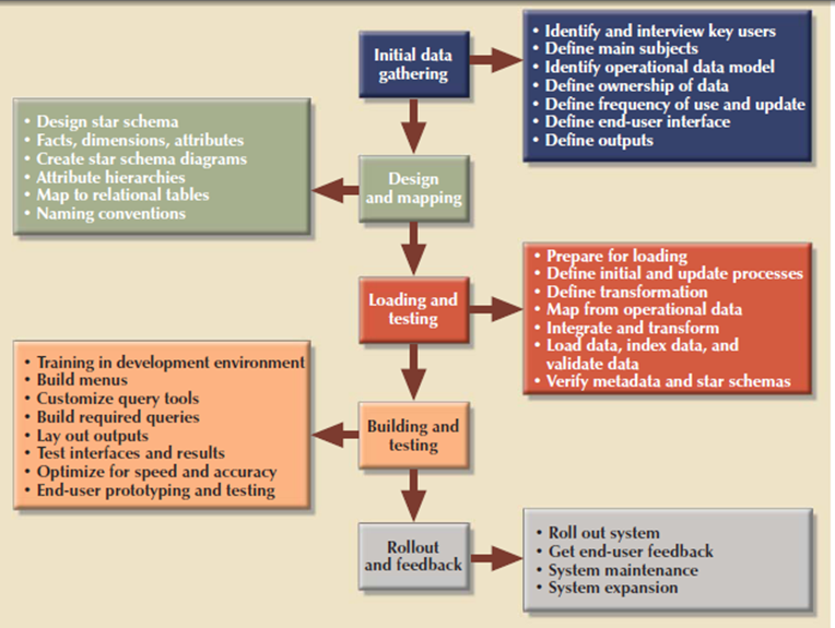
Figure 6.8 (I) Data warehouse design and implementation road map
The purpose of data analysis is to get previously unknown data characteristics, relationships, dependencies, or trends. Such discoveries are the part of the information framework on which decisions are built. A typical data analysis tool relies on the end users to define the problem, select the data, and initiate the acceptable data analyses to get the information that helps model and solve problems that the end users not find.
That means the end user reacts to an external stimulus the discovery of the problem itself. If the end user fails to detect a problem, no action is taken. Consider limitation some current BI environments now support various sorts of automated alerts.
The alerts are software agents that constantly monitor some parameters, like sales indicators and inventory levels, then perform specified actions (send e-mail or alert messages, run programs, then on) when these parameters reach predefined levels.
In contrast to the normal (reactive) BI tools, data mining is proactive. Rather than having the end user define the problem, select the information, and choose the tools to research the data, data-mining tools automatically search the info for anomalies and possible relationships, thereby identifying problems that haven't yet been identified by the top user.
In other words, data mining refers to the activities that analyze the info, uncover problems or opportunities hidden within the data relationships, form computer models supported their findings, then use the models to predict business behavior require minimal end-user intervention.
Therefore, the top user is in a position to use the system’s findings to achieve knowledge which may yield competitive advantages. Data mining describes a replacement breed of specialized decision support tools that automate data analysis. In short, data-mining tools initiate analyses to make knowledge.
Such knowledge are often used to address any number of business problems. For instance, banks and credit card companies use knowledge-based analysis to detect fraud, thereby decreasing fraudulent transactions.
Data mining represents how knowledge is extracted from data. Data form the pyramid base and represent what most organizations collect in their operational databases.
The second level contains information that represents the purified and processed data.
Information forms the idea for decision making and business understanding. Knowledge is found at the pyramid’s apex and represents highly specialized information.
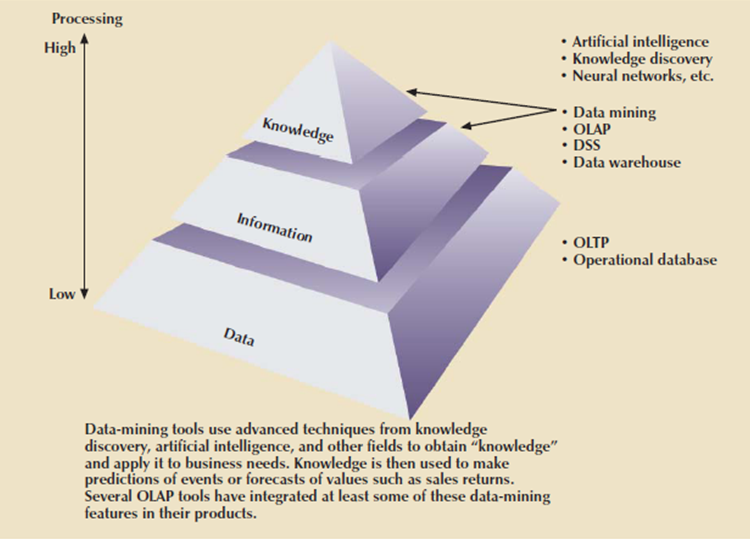
Figure 6.9(I) Extracting knowledge from data
It is difficult to supply a particular list of characteristics of data-mining tools. For one thing, the current generation of data-mining tools contains many design and application variations to suit data-mining requirements. Additionally, the various variations exist because there are not any established standards that govern the creation of data-mining tools.
Each data-mining tool seems to be governed by a special approach and focus, thus generating families of data-mining tools that specialize in market niches like marketing, retailing, finance, healthcare, investments, insurance, and banking.
Within a given niche, data-mining tools can use certain algorithms, and people algorithms are often implemented in several ways and/or applied over different data.
In spite of the shortage of precise standards, data mining is subject to four general phases:
1. Data preparation.
2. Data analysis and classification.
3. Knowledge acquisition.
4. Prognosis.
In the data preparation phase, the most data sets to be used by the data-mining operation are identified and cleansed of any data impurities. Because the information within the data warehouse are already integrated and filtered, the data warehouse usually is that the target set for data-mining operations.
The data analysis and classification phase used to identify common data characteristics or patterns. During this phase, the data-mining tool applies some algorithms to find:
• Data groupings, classifications, clusters, or sequences.
• Data dependencies, links, or relationships.
• Data patterns, trends, and deviations.
The knowledge acquisition phase uses the results of the data analysis and classification phase. During the knowledge acquisition phase, the data-mining tool selects the particular modeling or knowledge acquisition algorithms.
The common algorithms used in data mining are supported neural networks, decision trees, rules induction, genetic algorithms, classification and regression trees, memory-based reasoning, and nearest neighbor and data visualization. A data-mining tool use many of algorithms in any combination to get a computer model that reflects the behavior of the target data set.
Multiple data-mining tools stop at the knowledge-acquisition phase, others still in the prognosis phase. Therein phase, the data-mining findings are used to predict future behavior and forecast business outcomes. Following are the samples of data-mining findings are:
Sixty-five percent of consumers who didn't use credit card within the last six months are 88 percent to cancel that account.
Eighty-two percent of consumers who bought a 42-inch or larger LCD TV are 90 percent likely to shop for an entertainment center within subsequent four weeks. If age < 30 and income 25,000, then the minimum loan term is 10 years.
The complete set of findings are represented during a decision tree, a neural net, a forecasting model, or a visible presentation interface which is used to project future events or results. For instance, the prognosis phase might project the likely outcome of a new product rollout or a new marketing promotion. Figure shows the various phases of the data-mining techniques.
Because data-mining technology remains in its infancy, a number of the data-mining findings may fall outside the boundaries of what business managers expect. For instance, a data-mining tool might find a close relationship between a customer’s favorite brand of soda and therefore the brand of tires on the customer’s car. Clearly, that relationship won't be held in high regard among sales managers.
Fortunately, data mining usually yields more meaningful results. In fact, data mining has proved that it is helpful find practical relationships among data that help define customer buying patterns, improve product development and acceptance, reduce healthcare fraud, analyze stock markets, and many more.
Ideally, you'll expect the event of databases that not only store data and various statistics about data usage, but even have the ability to find out about and extract knowledge from the stored data. Such database management systems, also referred to as inductive or intelligent databases, are the main target of intense research in many laboratories.
Although those databases have yet to get claim to substantial commercial market penetration, both “add-on” and DBMS-integrated data-mining tools have proliferated within the data warehousing database market.
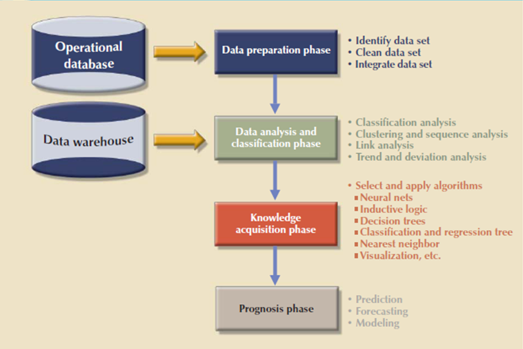
Figure 6.9(II) Data–mining phases
The proliferation of OLAP tools has fostered the development of SQL extensions to support multidimensional data analysis. Most SQL innovations are the results of vendor-centric product enhancements. However, many of the innovations have made their way into standard SQL. This section introduces a number of the new SQL extensions that are created to support OLAP-type data manipulations.
The SaleCo snowflake schema shown in above figure are used to demonstrate the use of the SQL extensions. This snowflake schema features a central DWSALESFACT fact table and three-dimension tables that is DWCUSTOMER, DWPRODUCT, and DWTIME. The central fact table shows daily sales by product and customer. Therefore the star schema shown in Figure see that the DWCUSTOMER and DWPRODUCT dimension tables have their own dimension tables: DWREGION and DWVENDOR.
A database is at the core of all data warehouses. Therefore, all SQL commands such as CREATE, INSERT, UPDATE, DELETE, and SELECT is work in the data warehouse as expected. Therefore the many queries run during a data warehouse include a lot of information groupings and aggregations over multiple columns. There are two extensions to the GROUP BY clause that are useful: ROLLUP and CUBE. Additionally, you'll study using materialized views to store preaggregated rows within the database.
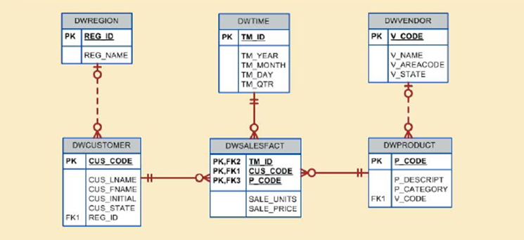
Figure 6.10(I) SaleCo snowflake schema 13.10.1
A. The ROLLUP Extension
The ROLLUP extension is worked with GROUP BY clause to get aggregates by different dimensions. The GROUP BY clause generate one aggregate for every new value combination of attributes listed within the GROUP BY clause. The ROLLUP extension goes one step next that it enables you to get a subtotal for every column listed apart from the last one, which gets a grand total instead. The syntax of the GROUP BY ROLLUP is as follows:
SELECT column1, column2 [, ...], aggregate_function(expression)
FROM table1 [,table2, _]
[WHERE condition]
GROUP BY ROLLUP (column1, column2 [, ...])
[HAVING condition]
[ORDER BY column1 [, column2, _]]
The order of the column list within the GROUP BY ROLLUP is extremely important. The last column within the list will generate a grand total. All other columns will generate subtotals. For instance, Figure shows the use of the ROLLUP extension to get subtotals by vendor and product.
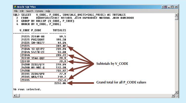
Figure 6.10(II) ROLLUP extension
Above figure shows the subtotals by vendor code and a grand total for all product codes. Contrast that with the traditional GROUP BY clause which will generate only the subtotals for every vendor and product combination instead of the subtotals by vendor and therefore the grand total for all products.
The ROLLUP extension is especially useful once you want to get multiple-nested subtotals for a dimension hierarchy. For instance, within a location hierarchy, you'll use ROLLUP to get subtotals by region, state, city, and store.
B. The CUBE Extension
The CUBE extension is used with the GROUP BY clause to find aggregates by the listed columns containing the last one. The CUBE extension used to calculate a subtotal for every column present within the expression, and a grand total for the last column listed. The syntax of the GROUP BY CUBE is as follows:
SELECT column1 [, column2, ...], aggregate_function(expression)
FROM table1 [,table2, _]
[WHERE condition]
GROUP BY CUBE (column1, column2 [, _])
[HAVING condition]
[ORDER BY column1 [, column2, _]]
For example, Figure shows the use of the CUBE extension to compute the sales subtotals by month and by product, also as a grand total.
The CUBE extension generates the subtotals for every combination of month and product, additionally to subtotals by month and by product, also as a grand total. The CUBE extension is especially useful once you want to compute all possible subtotals within groupings supported multiple dimensions. Cross-tabulations are especially good candidates for application of the CUBE extension.
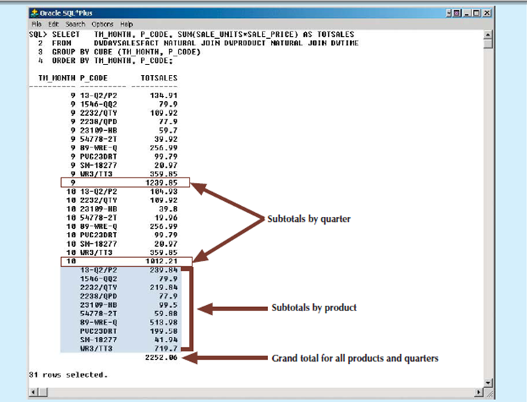
Figure 6.10(III) CUBE extension
C. Materialized Views
The data warehouse contains fact tables that store perticular measurements of interest to an organization. These measurements are organized by different dimensions. The ajority of OLAP business analysis of “everyday activities” is predicated on comparisons of information that are aggregated at different levels such as totals by vendor, by product, and by store.
Because businesses use a predefined set of summaries for benchmarking, it's reasonable to predefine such summaries for future use by creating summary fact tables. Creating multiple summary fact tables that use GROUP BY queries with multiple table joins become a resource-intensive operation.
Additionally, data warehouses need to maintain up-to-date summarized data in the least times. Therefore what happens with the summary fact tables after new sales data are added to the base fact tables? In normal circumstances, the summary fact tables are re-created. This operation needs the SQL code be run again to re-create all summary rows, even only a couple of rows needed updating. This is a time-consuming process.
To save query processing time database vendors implemented additional “functionality” to manage aggregate summaries efficiently. This new functionality resembles the standard SQL views that the SQL code is predefined within the database. However, the added functionality difference is that the views store the preaggregated rows, something sort of a summary table. For instance, Microsoft SQL Server provides indexed views and Oracle provides materialized views.
A materialized view is a dynamic table that contains the SQL query command to get the rows and stores the particular rows. The materialized view is made the first time the query is run and therefore the summary rows are stored within the table. The materialized view rows are automatically updated when the base tables are updated.
The data warehouse administrator create the view but no need to worry about updating the view. The utilization of materialized views is completely transparent to the end user. The OLAP end user can create OLAP queries, using the standard fact tables, and therefore the DBMS query optimization feature will automatically use the materialized views if those views provide better performance.
The basic syntax for the materialized view is:
CREATE MATERIALIZED VIEW view_name
BUILD {IMMEDIATE | DEFERRED}
REFRESH {[FAST | COMPLETE | FORCE]} ON COMMIT
[ENABLE QUERY REWRITE]
AS select_query;
The BUILD clause indicates when the materialized view rows are literally populated. IMMEDIATE indicates that the materialized view rows are populated after the command is entered. DEFERRED indicates that the materialized view rows are populated at a later time. The materialized view is in “unusable” state. The DBMS provides a special routine that an administrator runs to populate materialized views.
The REFRESH clause allows you to display when and the way to update the materialized view when new rows are added to the base tables. FAST indicates that whenever a change is formed within the base tables, the materialized view updates only the affected rows. COMPLETE indicates that an entire update are made for all rows within the materialized view when the select query on which the view is predicated is rerun.
FORCE represents that the DBMS will first attempt to do a quick update; otherwise do entire update. The ON COMMIT clause indicates that the updates to the materialized view will performed as a part of the commit process of the underlying DML statement is a part of the commitment of the DML transaction which updated the base tables. The ENABLE QUERY REWRITE option allows the DBMS to use the materialized views in query optimization.
To create materialized views, you need to have specified privileges and you want to complete specified prerequisite steps. You want to defer to the DBMS documentation for the newest updates. Within the case of Oracle, you want to create materialized view logs on the base tables of the materialized view.
Reference Book