2.1 Random variables | unit 2 probability distribution

Unit – 2

Probability Distribution

2.1 Random variables

Definition of Random Variable: A random variable is a variable whose possible values are the numerical outcomes of a random experiment. Therefore, it is a function which associate a unique numerical value with every outcome of an experiment. Further, its value varies with every trial of the experiment.

Random Variables:

A random variable is a numerical outcome of a random phenomenon.

For example: Flip three coins and let X represents the number of heads. X is a random variable.

We usually use capital letters to denotes random variables.

continuous random variable: A continuous random variable is a random variable where the data can take infinitely many values. For example, a random variable measuring the time taken for something to be done is continuous since there are an infinite number of possible times that can be taken.

Continuous random variable is called by a probability density function p (x), with given properties: p (x) ≥ 0 and the area between the x-axis& the curve is 1: ... standard deviation of a variable Random is defined by σ x = √Variance (x).

Properties

Starting from properties 1 to 7, c is a constant; x and y are random variables.

E(x + y) = E(x) + E(y).

E(cx) = c E(y).

Variance(x) = E(x2) - E(x)2

If x and y are individual, then Variance (x + y) = Variance(x) + Variance(y).

Variance(x + c) = Variance(x)

Variance(cx) = c2 Variance(x)

Co-variance(x + c, y) = Co-variance(x, y)

Co-variance(cx, y) = c Co-variance(x, y)

Co-variance(x, y + c) = Co-variance(x, y)

Co-variance(x, cy) = c Co-variance(x, y)

If x1, x2, ..., xn are discrete and N (μ, σ2), then E(x) = μ. We say that x is neutral for μ.

If x1, x2, ..., xn are independent and N (μ, σ2), then E(s) = σ2. We can tell S is neutral for σ2.

From given properties 8 to 12, w and v is random vector; b is a continuous vector; A is a continuous matrix.

8. E(v + w) = E(v) + E(w)

9. E(b) = b

10. E(Av) = A E(v)

11. Co-variance(v + b) = Co-variance(v)

12. Co-variance (Av) = A Co-variance(v) AT

Example 1: Consider tossing a fair coin 3 times.

Define X= the number of heads obtained.

Value	0	1	2	3
Probability	1/8	3/8	3/8	1/8

A: what is the probability of tossing at least two heads?

B: what is the probability of tossing fewer than three heads?

Solution:

X = 0, TTT

X = 1, HTT THT TTH

X = 2, HHT HTH THH

X = 3, HHH

A: Ans:

B: Ans:

(Or)

Example 2: Let the random variable X have probability density function

Find the cumulative distribution function of Y = g(x) =

Solution:

Example 3: Let X be a random variable with PDF given by

a. Find the constant c

b. Find EX and Var(X)

c. Find P(X)

Solution: a. To find c, We can use

Thus, we must have c=

b. To find EX, we can write

In fact, we could have guessed Ex=0 because the PDF is symmetric around x=0. To find Var(X), We have

c. To find P(X), we can write

Example 4: Let X be a continuous random variable with PDF given by

If Y =

Solution:

First, we note that

Thus,

Example 5: Let X be a continuous random variable with PDF

Find P(X).

Solution: We have

P(X) =

2.2 Discrete Probability distribution

Discrete Probability Distribution:

It describes the probability of occurrence of each value of a discrete random variable.

With Discrete Probability Distribution, each possible value of the discrete random variable can be associated with a non-zero probability

In the context of discrete variables.

Example 1: The probability distribution of a discrete random variable X is shown below.

X	1	2	3	4	5	6
Pr(X=x)	0.02	0.13	0.38	0.17	0.05	0.25

Find: a) Pr(X) b) Pr(X<5) c) Pr(X>0) d) Pr (2)

e) Pr(X)

Solution:

a): Pr(X) = Pr (X=0)+Pr(X=1)+Pr(X=2)+Pr(X=3)

= 0.02+0.13+0.38+0.17

= 0.7.

Working with Discrete Probability Distribution:

Example 2:

X	0	1	2	3	4 or more
P(X)	0.1	0.4	0.35	0.1	0.05

a): Verify that this is a legitimate probability distribution.

b): What is the probability that a customer does not rent any videos?

Solution:

a): Confirm that the sum of the probability is 1.

0.1+0.4+0.35+0.1+0.05 = 1

b): This is P(X=0) =0.1 or 10% of customer do not rent any videos.

Please notice the notation.

2.3 Continuous probability distribution

A probability distribution is a arithmetical function which defines completely possible values &possibilities that a random variable can take in a given range. This range will be bounded between the minimum and maximum possible values. But exactly where the possible value is possible to be plotted on the probability distribution depends on a number of influences. These factors include the distribution's mean, SD, skewness, and kurtosis.

Example 1: Following probability distribution

X	0	1	2	3	4	5	6	7
P(x)	0

Find: (i) k (ii)

(iii) Distribution function

(iv) If find minimum value of C

(v) Find

Solution:

If P(x) is p.m.f –

(i)

X	0	1	2	3	4	5	6	7
P(x)	0

(ii)

(iii)

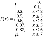
(iv)

(v)

Example 2: There are very few continuous distributions that we can do much with without a lot of math, but the simple uniform distribution is one of them. A uniform distribution is one that is just that-uniform. If we image any possible number between o and 2 as equally likely, we have an infinite possible number of numbers, so the probability of any particular number is close to zero. Instead of focusing on particular numbers, we have to focus on intervals.

The probability that some number between zero and two will come up will be one. To find the probability of any interval, we find the length of the interval and multiply by 5. Hence, the probability of getting a number between zero and one is 5.

For the following, draw the picture and compute the probabilities. What is:

a): P(0<x<.8)

b): P(x>.8)

c): P(.5<x<1.5)

d): P(.5<x<1.2) or P(.8<x<1.3)

e): compute the probability that we will not be in the interval of .4 to 1.5

f): compute the middle interval in which we will be 90% of the time.

g): compute the tails (outside intervals) that we will be in 5% of the time

Solution:

a): .8*.5 = .40

b): 1-.4 = .6

c): 1*.5 = .5

d): P(.5<x<1.5) = .8*.5 = .4

e): 1-P(.4<x<1.5) = 1-1.1*5 = 1-.55 = .45

f): 90% of 2 is 1.8, which centered will be from .1 to 1.9

g): 95% of the time we will be in the interval .05 to 1.95. 5% of the time we will

between 0 and .05 or 1.95 and 2.

Example 3: The picture below shows a continuous probability distribution with the formula, y = .5x for the range, x =0 to x = 2. In this case, area is probability.

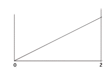
To compute the probability of being between 0 and 1, for example, you need to know y when x equals 1. The formula says it is .5. Hence, to find the probability that x is between 0 and 1 Prob(0<x<1), we compute the area of the triangle with a length of 1 and a height of .5. The answer is 2.5 because .5HW = .5*.5*1.

a). Show that the area under the line is equal to 1.

b). Find the following probabilities:

Prob(0<x<.5)

Prob(0<x<1.5)

Prob(1.5<x<2)

Prob(.5<x<1.5)

Prob (x<.5 or x>1.5)

c). Suppose that we draw twice from this distribution and that probability of the second draw is independent of the first. What is the probability of getting greater than 1.5 on both draws? What is the probability of getting less than 1.5 on both draws? What is the probability of getting a result greater than 1.5 on one draw and less than 1.5 on the other draw?

Solution:

a): Length *height*.5 is the area of a triangle. This triangle has length of 2 and height of 1, so 2*1*.5= 1. The area is one, and for a continuous distribution, area is probability.

b): Prob(0<x<.5)

Prob(0<x<.5) = .5*.5*.25 = .0625

Prob(0<x<1.5) = .5*1.5*.75 = .5625

Prob(1.5<x<2) = 1-Prob(0<x<1.5) = 1-.5625 = .4375.

Prob(.5<x<1.5) = .5625 - .0625 = .5

Prob (x<.5 or x>1.5) = .0625+.4375 = .5

c): Both less than 1.5: .5625*.5625 = .3164: both greater than 1.5: .4375*.4375 = .1914; one greater and one less: 1 - .3164 - .1914 = .4922.

2.4 Binomial Distribution

A distribution is said to be binomial distribution if the following conditions are met.

Each trial has a binary outcome (One of the two outcomes is labelled a ‘success’)

The probability of success is known and constant over all trials

The number of trials is specified

The trials are independent. That is, the outcome from one trial doesn’t affect the outcome of successive trials

If all the above conditions met then the binomial distribution describes the probability of X successes in n trials.

A classic example of the binomial distribution is the number of heads (X) in n coin tosses.

The Notation for a binomial distribution is

X ~ B (n, π)

which is read as ‘X is distributed binomial with n trials and probability of success in one trial equal to π’.

formula for binomial distribution:

Using this formula, the probability distribution of a binomial random variable X can be calculated if n and π are known.

p(x) =

n! is called ‘n factorial’ = n(n-1)(n-2) . . .(1)

P(X) = #of Scenario * Single Scenario

The first factorial terms gives the number of scenario and the second term describes the probability of success to power of number of successes and probability of failure to the power of number of failures.

Binomial Distribution-Mean and Variance:

Any random variable with a binomial distribution X with parameters n and p is a sum of n independent Bernoulli random variables in which the probability of success is p.

The mean and variance of each

can easily be calculated as:

Hence the mean and variance of X are given by (remember the

are independent)

Example 1: Jean usually makes half of her free throws in basketball practice. Today, she tries 3 free throws. What is the probability that Jean will make exactly 1 of her free throws?

Solution: The Probability that Jean will make each free throw is or 0.5.

P(r) = Substitute 3 for n, 1 for r, 0.5 for p, and 0.5 for q

P (1) =

= 3(0.5)(0.25) = 0.375

The probability that Jean will make exactly one free throw is 37.5%.

Example 2: Suppose the probability of purchasing a defective computer is 0.02. What is the probability of purchasing 2 defective computers in a group of 10?

X = 2, n = 10, and

Solution: P(X=2) =

= (45)(0.0004)(0.8508)

= 0.01531

Example 3: A dozen eggs contain 3 defectives. If a sample of 5 is taken with replacement, find the probability that.

a) Exactly 2 of the eggs sampled are defective.

b) 2 or fewer of the eggs sampled are defective

Solution: If n = 5, P = ¼

“Success = Defective”

x = 0,1,2,3,4,5

f(x) =

P(X=2) = f(2)=

P(X

2.5 Poisson Distribution

Examples of events over space or time: -number of cells in a specified volume of fluid

-number of calls/hours to a help line

-number of emergency room beds filled/ 24 hours

Like the binomial distribution and the normal distribution, there are many Poisson distributions.

Each Poisson distribution is specified by the average rate at which the event occurs.

The rate is notated with λ

λ = ‘lambda’, Greek letter ‘L’– There is only one parameter for the Poisson distribution

The probability that there are exactly X occurrences in the specified space or time is equal to

p(x) =

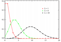
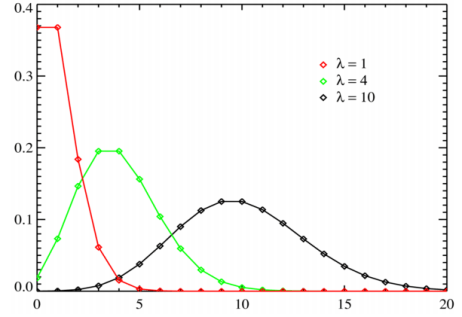
The horizontal axis is the index X. The function is defined only at integer values of X. The connecting lines are only guiding for the eye and do not indicate continuity. Notice that as λ increases the distribution begins to resemble a normal distribution.

If λ is 10 or greater, the normal distribution is a reasonable approximation to the Poisson distribution

The mean and variance for a Poisson distribution are the same and are both equal to λ

The standard deviation of the Poisson distribution is the square root of λ

Mean and Variance for the Poisson Distribution:

It’s easy to show that for this distribution,

The Mean is:

The Variance is:

So, the standard deviation is .

Example 1: Suppose that a rare disease has an incidence of 1 in 1000 person-years. Assuming that members of the population are affected independently, find the probability of k cases in a population of 10,000(followed over 1 year) for k=0,1,2.

Solution: The expected value (mean)

10 new cases expected in this population per year

Example 2: Suppose that the probability of a defect in a foot of magnetic tape is 0.002. Use the Poisson distribution to compute the probability that 1500 feet roll will have no defects.

Solution:

2.6 Normal Distribution

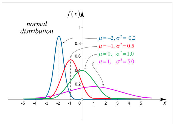
The normal distribution is the utmost broadly identified P.D. then it defines many usual spectacles.

The PDF of the normal distribution is shown by method

f(x)=,

where μ is mean of the distribution, and is the variance.

The 2 limitations μ and σ completely describe the figure and all additional things of the normal distribution function.

Properties of normal distribution:

The mean, mode and median are all equal.

The curve is symmetric at the center (i.e. around the mean, μ).

Exactly half of the values are to the left of center and exactly half the values are to the right.

The total area under the curve is 1.

Example 1: The weekly incomes of shit foremen in the glass industry follow the normal probability distribution with a mean of $1,000 and a standard deviation of $ 100. What is the z value for the income, let’s call it X, of a foreman who earns $1,100 per week? For a foreman who earns $900 per week?

Solution: For X = $ 1,100: