UNIT- 5
Trees
Tree

Basic terminology
Static representation of tree
Dynamic representation of tree
Types of Tree
The tree data structure can be classified into six different categories.

General Tree
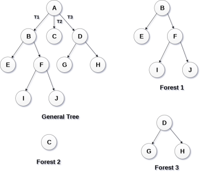
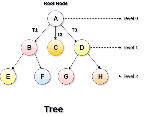
General Tree stores the elements in a hierarchical order in which the top level element is always present at level 0 as the root element. All the nodes except the root node are present at number of levels. The nodes which are present on the same level are called siblings while the nodes which are present on the different levels exhibit the parent-child relationship among them. A node may contain any number of sub-trees. The tree in which each node contain 3 sub-tree, is called ternary tree.
Forests
Forest can be defined as the set of disjoint trees which can be obtained by deleting the root node and the edges which connects root node to the first level node.
Binary Tree
Binary tree is a data structure in which each node can have at most 2 children. The node present at the top most level is called the root node. A node with the 0 children is called leaf node. Binary Trees are used in the applications like expression evaluation and many more. We will discuss binary tree in detail, later in this tutorial.
Binary Search Tree
Binary search tree is an ordered binary tree. All the elements in the left sub-tree are less than the root while elements present in the right sub-tree are greater than or equal to the root node element. Binary search trees are used in most of the applications of computer science domain like searching, sorting, etc.
Expression Tree
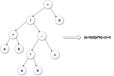
Expression trees are used to evaluate the simple arithmetic expressions. Expression tree is basically a binary tree where internal nodes are represented by operators while the leaf nodes are represented by operands. Expression trees are widely used to solve algebraic expressions like (a+b)*(a-b). Consider the following example.
Q. Construct an expression tree by using the following algebraic expression.
(a + b) / (a*b - c) + d
Tournament Tree
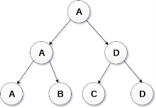
Tournament tree are used to record the winner of the match in each round being played between two players. Tournament tree can also be called as selection tree or winner tree. External nodes represent the players among which a match is being played while the internal nodes represent the winner of the match played. At the top most level, the winner of the tournament is present as the root node of the tree.
For example, tree .of a chess tournament being played among 4 players is shown as follows. However, the winner in the left sub-tree will play against the winner of right sub-tree.
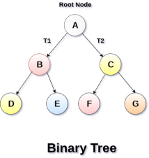
Binary Tree is a special type of generic tree in which, each node can have at most two children. Binary tree is generally partitioned into three disjoint subsets.
A binary Tree is shown in the following image.
Types of Binary Tree
1. Strictly Binary Tree
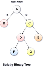
In Strictly Binary Tree, every non-leaf node contain non-empty left and right sub-trees. In other words, the degree of every non-leaf node will always be 2. A strictly binary tree with n leaves, will have (2n - 1) nodes.
A strictly binary tree is shown in the following figure.
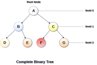
2. Complete Binary Tree
A Binary Tree is said to be a complete binary tree if all of the leaves are located at the same level d. A complete binary tree is a binary tree that contains exactly 2^l nodes at each level between level 0 and d. The total number of nodes in a complete binary tree with depth d is 2d+1-1 where leaf nodes are 2d while non-leaf nodes are 2d-1.
Binary Tree Traversal
SN | Traversal | Description |
1 | Pre-order Traversal | Traverse the root first then traverse into the left sub-tree and right sub-tree respectively. This procedure will be applied to each sub-tree of the tree recursively. |
2 | In-order Traversal | Traverse the left sub-tree first, and then traverse the root and the right sub-tree respectively. This procedure will be applied to each sub-tree of the tree recursively. |
3 | Post-order Traversal | Traverse the left sub-tree and then traverse the right sub-tree and root respectively. This procedure will be applied to each sub-tree of the tree recursively. |
Binary Tree representation
There are two types of representation of a binary tree:
1. Linked Representation
In this representation, the binary tree is stored in the memory, in the form of a linked list where the number of nodes are stored at non-contiguous memory locations and linked together by inheriting parent child relationship like a tree. every node contains three parts : pointer to the left node, data element and pointer to the right node. Each binary tree has a root pointer which points to the root node of the binary tree. In an empty binary tree, the root pointer will point to null.
Consider the binary tree given in the figure below.
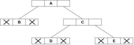
In the above figure, a tree is seen as the collection of nodes where each node contains three parts : left pointer, data element and right pointer. Left pointer stores the address of the left child while the right pointer stores the address of the right child. The leaf node contains null in its left and right pointers.
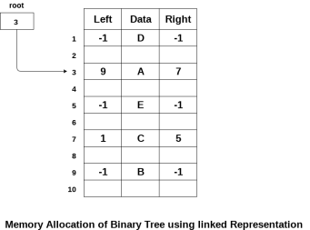
The following image shows about how the memory will be allocated for the binary tree by using linked representation. There is a special pointer maintained in the memory which points to the root node of the tree. Every node in the tree contains the address of its left and right child. Leaf node contains null in its left and right pointers.
2. Sequential Representation
This is the simplest memory allocation technique to store the tree elements but it is an inefficient technique since it requires a lot of space to store the tree elements. A binary tree is shown in the following figure along with its memory allocation.
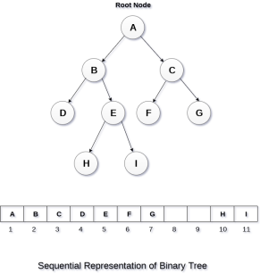
In this representation, an array is used to store the tree elements. Size of the array will be equal to the number of nodes present in the tree. The root node of the tree will be present at the 1st index of the array. If a node is stored at ith index then its left and right children will be stored at 2i and 2i+1 location. If the 1st index of the array i.e. tree[1] is 0, it means that the tree is empty.
Traversal is a process to visit all the nodes of a tree and may print their values too. Because, all nodes are connected via edges (links) we always start from the root (head) node. That is, we cannot randomly access a node in a tree. There are three ways which we use to traverse a tree −
Generally, we traverse a tree to search or locate a given item or key in the tree or to print all the values it contains.
In-order Traversal
In this traversal method, the left subtree is visited first, then the root and later the right sub-tree. We should always remember that every node may represent a subtree itself.
If a binary tree is traversed in-order, the output will produce sorted key values in an ascending order.
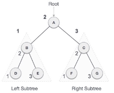
We start from A, and following in-order traversal, we move to its left subtree B. B is also traversed in-order. The process goes on until all the nodes are visited. The output of inorder traversal of this tree will be −
D → B → E →A→ F → C → G
Algorithm
Until all nodes are traversed −
Step 1− Recursively traverse left subtree.
Step 2− Visit root node.
Step 3− Recursively traverse right subtree.
Pre-order Traversal
In this traversal method, the root node is visited first, then the left subtree and finally the right subtree.
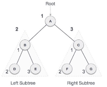
We start from A, and following pre-order traversal, we first visit A itself and then move to its left subtree B. B is also traversed pre-order. The process goes on until all the nodes are visited. The output of pre-order traversal of this tree will be −
A → B → D → E → C → F → G
Algorithm
Until all nodes are traversed −
Step 1− Visit root node.
Step 2− Recursively traverse left subtree.
Step 3− Recursively traverse right subtree.
Post-order Traversal
In this traversal method, the root node is visited last, hence the name. First we traverse the left subtree, then the right subtree and finally the root node.
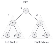
We start from A, and following Post-order traversal, we first visit the left subtree B. B is also traversed post-order. The process goes on until all the nodes are visited. The output of post-order traversal of this tree will be −
D → E → B → F → G → C → A
Algorithm
Until all nodes are traversed −
Step 1− Recursively traverse left subtree.
Step 2− Recursively traverse right subtree.
Step 3− Visit root node.
To check the C implementation of tree traversing, please.
Tree Traversal in C
Traversal is a process to visit all the nodes of a tree and may print their values too. Because, all nodes are connected via edges (links) we always start from the root (head) node. That is, we cannot random access a node in a tree. There are three ways which we use to traverse a tree −
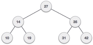
We shall now look at the implementation of tree traversal in C programming language here using the following binary tree −
Implementation in C
#include <stdio.h>
#include <stdlib.h>
struct node {
int data;
struct node *leftChild;
struct node *rightChild;
};
struct node *root = NULL;
void insert(int data) {
struct node *tempNode = (struct node*) malloc(sizeof(struct node));
struct node *current;
struct node *parent;
tempNode->data = data;
tempNode->leftChild = NULL;
tempNode->rightChild = NULL;
//if tree is empty
if(root == NULL) {
root = tempNode;
} else {
current = root;
parent = NULL;
while(1) {
parent = current;
//go to left of the tree
if(data < parent->data) {
current = current->leftChild;
//insert to the left
if(current == NULL) {
parent->leftChild = tempNode;
return;
}
} //go to right of the tree
else {
current = current->rightChild;
//insert to the right
if(current == NULL) {
parent->rightChild = tempNode;
return;
}
}
}
}
}
struct node* search(int data) {
struct node *current = root;
printf("Visiting elements: ");
while(current->data != data) {
if(current != NULL)
printf("%d ",current->data);
//go to left tree
if(current->data > data) {
current = current->leftChild;
}
//else go to right tree
else {
current = current->rightChild;
}
//not found
if(current == NULL) {
return NULL;
}
}
return current;
}
voidpre_order_traversal(struct node* root) {
if(root != NULL) {
printf("%d ",root->data);
pre_order_traversal(root->leftChild);
pre_order_traversal(root->rightChild);
}
}
voidinorder_traversal(struct node* root) {
if(root != NULL) {
inorder_traversal(root->leftChild);
printf("%d ",root->data);
inorder_traversal(root->rightChild);
}
}
voidpost_order_traversal(struct node* root) {
if(root != NULL) {
post_order_traversal(root->leftChild);
post_order_traversal(root->rightChild);
printf("%d ", root->data);
}
}
int main() {
inti;
int array[7] = { 27, 14, 35, 10, 19, 31, 42 };
for(i = 0; i< 7; i++)
insert(array[i]);
i = 31;
struct node * temp = search(i);
if(temp != NULL) {
printf("[%d] Element found.", temp->data);
printf("\n");
}else {
printf("[ x ] Element not found (%d).\n", i);
}
i = 15;
temp = search(i);
if(temp != NULL) {
printf("[%d] Element found.", temp->data);
printf("\n");
}else {
printf("[ x ] Element not found (%d).\n", i);
}
printf("\nPreorder traversal: ");
pre_order_traversal(root);
printf("\nInorder traversal: ");
inorder_traversal(root);
printf("\nPost order traversal: ");
post_order_traversal(root);
return 0;
}
If we compile and run the above program, it will produce the following result −
Output
Visiting elements: 27 35 [31] Element found.
Visiting elements: 27 14 19 [ x ] Element not found (15).
Preorder traversal: 27 14 10 19 35 31 42
Inorder traversal: 10 14 19 27 31 35 42
Post order traversal: 10 19 14 31 42 35 27
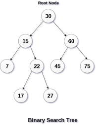
A Binary search tree is shown in the above figure. As the constraint applied on the BST, we can see that the root node 30 doesn't contain any value greater than or equal to 30 in its left sub-tree and it also doesn't contain any value less than 30 in its right sub-tree.
Advantages of using binary search tree
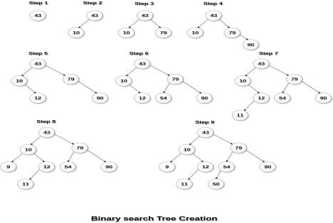
Q. Create the binary search tree using the following data elements.
43, 10, 79, 90, 12, 54, 11, 9, 50
The process of creating BST by using the given elements, is shown in the image below.
Operations on Binary Search Tree
There are many operations which can be performed on a binary search tree.
SN | Operation | Description |
1 | Searching in BST | Finding the location of some specific element in a binary search tree. |
2 | Insertion in BST | Adding a new element to the binary search tree at the appropriate location so that the property of BST do not violate. |
3 | Deletion in BST | Deleting some specific node from a binary search tree. However, there can be various cases in deletion depending upon the number of children, the node have. |
Program to implement BST operations
Output:
Enter value to be inserted? 10
Enter value to be inserted? 20
Enter value to be inserted? 30
Enter value to be inserted? 40
Enter value to be inserted? 5
Enter value to be inserted? 25
Enter value to be inserted? 15
Enter value to be inserted? 5
5 5 10 15 20 25 30 40
5 5 15 20 25 30 40
AVL Tree is invented by GM Adelson - Velsky and EM Landis in 1962. The tree is named AVL in honour of its inventors.
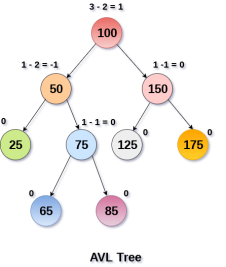
AVL Tree can be defined as height balanced binary search tree in which each node is associated with a balance factor which is calculated by subtracting the height of its right sub-tree from that of its left sub-tree.
Tree is said to be balanced if balance factor of each node is in between -1 to 1, otherwise, the tree will be unbalanced and need to be balanced.
Balance Factor (k) = height (left(k)) - height (right(k))
If balance factor of any node is 1, it means that the left sub-tree is one level higher than the right sub-tree.
If balance factor of any node is 0, it means that the left sub-tree and right sub-tree contain equal height.
If balance factor of any node is -1, it means that the left sub-tree is one level lower than the right sub-tree.
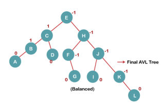
An AVL tree is given in the following figure. We can see that, balance factor associated with each node is in between -1 and +1. therefore, it is an example of AVL tree.
Complexity
Algorithm | Average case | Worst case |
Space | o(n) | o(n) |
Search | o(log n) | o(log n) |
Insert | o(log n) | o(log n) |
Delete | o(log n) | o(log n) |
Operations on AVL tree
Due to the fact that, AVL tree is also a binary search tree therefore, all the operations are performed in the same way as they are performed in a binary search tree. Searching and traversing do not lead to the violation in property of AVL tree. However, insertion and deletion are the operations which can violate this property and therefore, they need to be revisited.
SN | Operation | Description |
1 | Insertion | Insertion in AVL tree is performed in the same way as it is performed in a binary search tree. However, it may lead to violation in the AVL tree property and therefore the tree may need balancing. The tree can be balanced by applying rotations. |
2 | Deletion | Deletion can also be performed in the same way as it is performed in a binary search tree. Deletion may also disturb the balance of the tree therefore, various types of rotations are used to rebalance the tree. |
Why AVL Tree?
AVL tree controls the height of the binary search tree by not letting it to be skewed. The time taken for all operations in a binary search tree of height h is O(h). However, it can be extended to O(n) if the BST becomes skewed (i.e. worst case). By limiting this height to log n, AVL tree imposes an upper bound on each operation to be O(log n) where n is the number of nodes.
AVL Rotations
We perform rotation in AVL tree only in case if Balance Factor is other than -1, 0, and 1. There are basically four types of rotations which are as follows:
Where node A is the node whose balance Factor is other than -1, 0, 1.
The first two rotations LL and RR are single rotations and the next two rotations LR and RL are double rotations. For a tree to be unbalanced, minimum height must be at least 2, Let us understand each rotation
1. RR Rotation
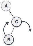
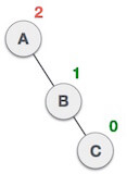
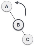
When BST becomes unbalanced, due to a node is inserted into the right subtree of the right subtree of A, then we perform RR rotation, RR rotation is an anticlockwise rotation, which is applied on the edge below a node having balance factor -2
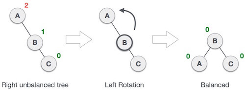
In above example, node A has balance factor -2 because a node C is inserted in the right subtree of A right subtree. We perform the RR rotation on the edge below A.
2. LL Rotation
When BST becomes unbalanced, due to a node is inserted into the left subtree of the left subtree of C, then we perform LL rotation, LL rotation is clockwise rotation, which is applied on the edge below a node having balance factor 2.
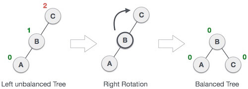
In above example, node C has balance factor 2 because a node A is inserted in the left subtree of C left subtree. We perform the LL rotation on the edge below A.
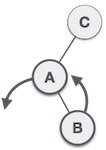
3. LR Rotation
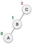
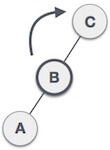
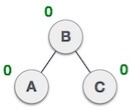
Double rotations are bit tougher than single rotation which has already explained above. LR rotation = RR rotation + LL rotation, i.e., first RR rotation is performed on subtree and then LL rotation is performed on full tree, by full tree we mean the first node from the path of inserted node whose balance factor is other than -1, 0, or 1.
Let us understand each and every step very clearly:
State | Action |
| A node B has been inserted into the right subtree of A the left subtree of C, because of which C has become an unbalanced node having balance factor 2. This case is L R rotation where: Inserted node is in the right subtree of left subtree of C |
| As LR rotation = RR + LL rotation, hence RR (anticlockwise) on subtree rooted at A is performed first. By doing RR rotation, node A, has become the left subtree of B. |
| After performing RR rotation, node C is still unbalanced, i.e., having balance factor 2, as inserted node A is in the left of left of C |
| Now we perform LL clockwise rotation on full tree, i.e. on node C. node C has now become the right subtree of node B, A is left subtree of B |
| Balance factor of each node is now either -1, 0, or 1, i.e. BST is balanced now. |
4. RL Rotation
As already discussed, that double rotations are bit tougher than single rotation which has already explained above. R L rotation = LL rotation + RR rotation, i.e., first LL rotation is performed on subtree and then RR rotation is performed on full tree, by full tree we mean the first node from the path of inserted node whose balance factor is other than -1, 0, or 1.
State | Action |
| A node B has been inserted into the left subtree of C the right subtree of A, because of which A has become an unbalanced node having balance factor - 2. This case is RL rotation where: Inserted node is in the left subtree of right subtree of A |
| As RL rotation = LL rotation + RR rotation, hence, LL (clockwise) on subtree rooted at C is performed first. By doing RR rotation, node C has become the right subtree of B. |
| After performing LL rotation, node A is still unbalanced, i.e. having balance factor -2, which is because of the right-subtree of the right-subtree node A. |
| Now we perform RR rotation (anticlockwise rotation) on full tree, i.e. on node A. node C has now become the right subtree of node B, and node A has become the left subtree of B. |
| Balance factor of each node is now either -1, 0, or 1, i.e., BST is balanced now. |
Q: Construct an AVL tree having the following elements
H, I, J, B, A, E, C, F, D, G, K, L
1. Insert H, I, J
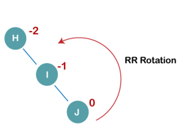
On inserting the above elements, especially in the case of H, the BST becomes unbalanced as the Balance Factor of H is -2. Since the BST is right-skewed, we will perform RR Rotation on node H.
The resultant balance tree is:
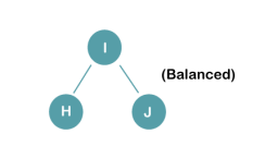
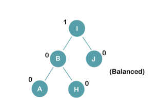
2. Insert B, A
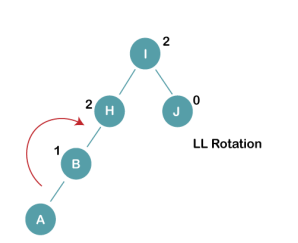
On inserting the above elements, especially in case of A, the BST becomes unbalanced as the Balance Factor of H and I is 2, we consider the first node from the last inserted node i.e. H. Since the BST from H is left-skewed, we will perform LL Rotation on node H.
The resultant balance tree is:
3. Insert E
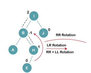
On inserting E, BST becomes unbalanced as the Balance Factor of I is 2, since if we travel from E to I we find that it is inserted in the left subtree of right subtree of I, we will perform LR Rotation on node I. LR = RR + LL rotation
3 a) We first perform RR rotation on node B
The resultant tree after RR rotation is:
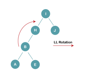
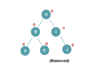
3b) We first perform LL rotation on the node I
The resultant balanced tree after LL rotation is:
4. Insert C, F, D
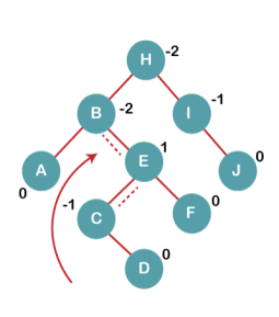
On inserting C, F, D, BST becomes unbalanced as the Balance Factor of B and H is -2, since if we travel from D to B we find that it is inserted in the right subtree of left subtree of B, we will perform RL Rotation on node I. RL = LL + RR rotation.
4a) We first perform LL rotation on node E
The resultant tree after LL rotation is:
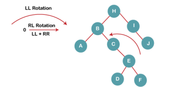
4b) We then perform RR rotation on node B
The resultant balanced tree after RR rotation is:
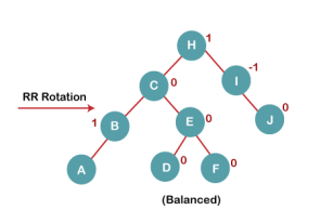
5. Insert G
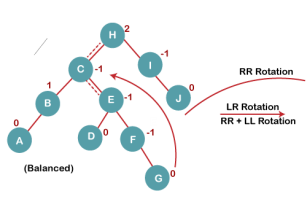
On inserting G, BST become unbalanced as the Balance Factor of H is 2, since if we travel from G to H, we find that it is inserted in the left subtree of right subtree of H, we will perform LR Rotation on node I. LR = RR + LL rotation.
5 a) We first perform RR rotation on node C
The resultant tree after RR rotation is:
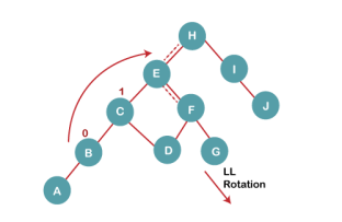
5 b) We then perform LL rotation on node H
The resultant balanced tree after LL rotation is:
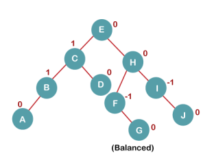
6. Insert K
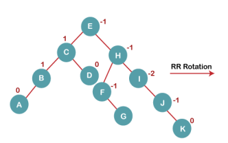
On inserting K, BST becomes unbalanced as the Balance Factor of I is -2. Since the BST is right-skewed from I to K, hence we will perform RR Rotation on the node I.
The resultant balanced tree after RR rotation is:
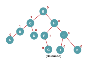
7. Insert L
On inserting the L tree is still balanced as the Balance Factor of each node is now either, -1, 0, +1. Hence the tree is a Balanced AVL tree
B Tree
B Tree is a specialized m-way tree that can be widely used for disk access. A B-Tree of order m can have at most m-1 keys and m children. One of the main reason of using B tree is its capability to store large number of keys in a single node and large key values by keeping the height of the tree relatively small.
A B tree of order m contains all the properties of an M way tree. In addition, it contains the following properties.
It is not necessary that, all the nodes contain the same number of children but, each node must have m/2 number of nodes.
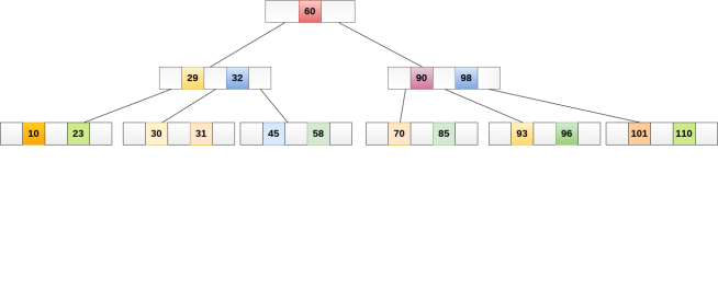
A B tree of order 4 is shown in the following image.
While performing some operations on B Tree, any property of B Tree may violate such as number of minimum children a node can have. To maintain the properties of B Tree, the tree may split or join.
Operations
Searching :
Searching in B Trees is similar to that in Binary search tree. For example, if we search for an item 49 in the following B Tree. The process will something like following :
Searching in a B tree depends upon the height of the tree. The search algorithm takes O(log n) time to search any element in a B tree.
Inserting
Insertions are done at the leaf node level. The following algorithm needs to be followed in order to insert an item into B Tree.
- Insert the new element in the increasing order of elements.
- Split the node into the two nodes at the median.
- Push the median element upto its parent node.
- If the parent node also contain m-1 number of keys, then split it too by following the same steps.
Example:
Insert the node 8 into the B Tree of order 5 shown in the following image.

8 will be inserted to the right of 5, therefore insert 8.

The node, now contain 5 keys which is greater than (5 -1 = 4 ) keys. Therefore split the node from the median i.e. 8 and push it up to its parent node shown as follows.

Deletion
Deletion is also performed at the leaf nodes. The node which is to be deleted can either be a leaf node or an internal node. Following algorithm needs to be followed in order to delete a node from a B tree.
- If the left sibling contains more than m/2 elements then push its largest element up to its parent and move the intervening element down to the node where the key is deleted.
- If the right sibling contains more than m/2 elements then push its smallest element up to the parent and move intervening element down to the node where the key is deleted.
If the the node which is to be deleted is an internal node, then replace the node with its in-order successor or predecessor. Since, successor or predecessor will always be on the leaf node hence, the process will be similar as the node is being deleted from the leaf node.
Example 1
Delete the node 53 from the B Tree of order 5 shown in the following figure.

53 is present in the right child of element 49. Delete it.

Now, 57 is the only element which is left in the node, the minimum number of elements that must be present in a B tree of order 5, is 2. it is less than that, the elements in its left and right sub-tree are also not sufficient therefore, merge it with the left sibling and intervening element of parent i.e. 49.
The final B tree is shown as follows.

Application of B tree
B tree is used to index the data and provides fast access to the actual data stored on the disks since, the access to value stored in a large database that is stored on a disk is a very time consuming process.
Searching an un-indexed and unsorted database containing n key values needs O(n) running time in worst case. However, if we use B Tree to index this database, it will be searched in O(log n) time in worst case.
B+ Tree
B+ Tree is an extension of B Tree which allows efficient insertion, deletion and search operations.
In B Tree, Keys and records both can be stored in the internal as well as leaf nodes. Whereas, in B+ tree, records (data) can only be stored on the leaf nodes while internal nodes can only store the key values.
The leaf nodes of a B+ tree are linked together in the form of a singly linked lists to make the search queries more efficient.
B+ Tree are used to store the large amount of data which can not be stored in the main memory. Due to the fact that, size of main memory is always limited, the internal nodes (keys to access records) of the B+ tree are stored in the main memory whereas, leaf nodes are stored in the secondary memory.
The internal nodes of B+ tree are often called index nodes. A B+ tree of order 3 is shown in the following figure.

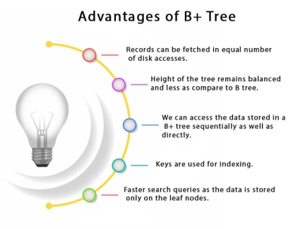
Advantages of B+ Tree
B Tree VS B+ Tree
SN | B Tree | B+ Tree |
1 | Search keys can not be repeatedly stored. | Redundant search keys can be present. |
2 | Data can be stored in leaf nodes as well as internal nodes | Data can only be stored on the leaf nodes. |
3 | Searching for some data is a slower process since data can be found on internal nodes as well as on the leaf nodes. | Searching is comparatively faster as data can only be found on the leaf nodes. |
4 | Deletion of internal nodes are so complicated and time consuming. | Deletion will never be a complexed process since element will always be deleted from the leaf nodes. |
5 | Leaf nodes can not be linked together. | Leaf nodes are linked together to make the search operations more efficient. |
Insertion in B+ Tree
Step 1: Insert the new node as a leaf node
Step 2: If the leaf doesn't have required space, split the node and copy the middle node to the next index node.
Step 3: If the index node doesn't have required space, split the node and copy the middle element to the next index page.
Example :
Insert the value 195 into the B+ tree of order 5 shown in the following figure.

195 will be inserted in the right sub-tree of 120 after 190. Insert it at the desired position.

The node contains greater than the maximum number of elements i.e. 4, therefore split it and place the median node up to the parent.

Now, the index node contains 6 children and 5 keys which violates the B+ tree properties, therefore we need to split it, shown as follows.

Deletion in B+ Tree
Step 1: Delete the key and data from the leaves.
Step 2: if the leaf node contains less than minimum number of elements, merge down the node with its sibling and delete the key in between them.
Step 3: if the index node contains less than minimum number of elements, merge the node with the sibling and move down the key in between them.
Example
Delete the key 200 from the B+ Tree shown in the following figure.

200 is present in the right sub-tree of 190, after 195. delete it.

Merge the two nodes by using 195, 190, 154 and 129.

Now, element 120 is the single element present in the node which is violating the B+ Tree properties. Therefore, we need to merge it by using 60, 78, 108 and 120.
Now, the height of B+ tree will be decreased by 1.

Heap data structure is a complete binary tree that satisfies the heap property. It is also called as a binary heap.
A complete binary tree is a special binary tree in which
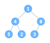
Heap Property is the property of a node in which

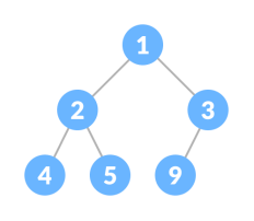
Heap Operations
Some of the important operations performed on a heap are described below along with their algorithms.
Heapify
Heapify is the process of creating a heap data structure from a binary tree. It is used to create a Min-Heap or a Max-Heap.

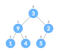
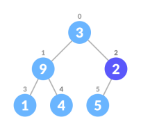
If leftChild is greater than currentElement (i.e. element at ith index), set leftChildIndex as largest.
If rightChild is greater than element in largest, set rightChildIndex as largest.
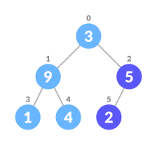
Algorithm
Heapify(array, size, i)
setias largest
leftChild = 2i + 1
rightChild = 2i + 2
ifleftChild> array[largest]
setleftChildIndexas largest
ifrightChild> array[largest]
setrightChildIndexas largest
swaparray[i] andarray[largest]
To create a Max-Heap:
MaxHeap(array, size)
loopfrom the first index of non-leaf node down to zero
callheapify
For Min-Heap, both leftChild and rightChild must be smaller than the parent for all nodes.
Insert Element into Heap
Algorithm for insertion in Max Heap
If there is no node,
create a newNode.
else (a node is already present)
insert the newNodeat the end (last node fromleftto right.)
heapify the array
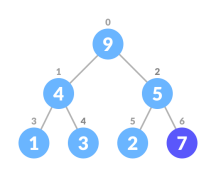
2. Heapify the tree.
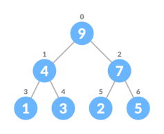
For Min Heap, the above algorithm is modified so that parentNode is always smaller than newNode.
Delete Element from Heap
Algorithm for deletion in Max Heap
IfnodeToBeDeleted is the leafNode
removethe node
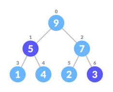
Elseswap nodeToBeDeleted with the lastLeafNode
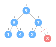
removenoteToBeDeleted
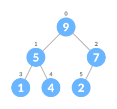
heapifythe array
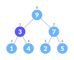
2. Swap it with the last element.
3. Remove the last element.
4. Heapify the tree.
For Min Heap, above algorithm is modified so that both childNodes are greater smaller than currentNode.
Peek (Find max/min)
Peek operation returns the maximum element from Max Heap or minimum element from Min Heap without deleting the node.
For both Max heap and Min Heap
returnrootNode
Extract-Max/Min
Extract-Max returns the node with maximum value after removing it from a Max Heap whereas Extract-Min returns the node with minimum after removing it from Min Heap.
Python, Java, C/C++ Examples
# Max-Heap data structure in Python
defheapify(arr, n, i):
largest = i
l = 2 * i + 1
r = 2 * i + 2
if l < n andarr[i] <arr[l]:
largest = l
if r < n andarr[largest] <arr[r]:
largest = r
if largest != i:
arr[i],arr[largest] = arr[largest],arr[i]
heapify(arr, n, largest)
definsert(array, newNum):
size = len(array)
if size == 0:
array.append(newNum)
else:
array.append(newNum);
foriin range((size//2)-1, -1, -1):
heapify(array, size, i)
defdeleteNode(array, num):
size = len(array)
i = 0
foriin range(0, size):
ifnum == array[i]:
break
array[i], array[size-1] = array[size-1], array[i]
array.remove(size-1)
foriin range((len(array)//2)-1, -1, -1):
heapify(array, len(array), i)
arr = []
insert(arr, 3)
insert(arr, 4)
insert(arr, 9)
insert(arr, 5)
insert(arr, 2)
print ("Max-Heap array: " + str(arr))
deleteNode(arr, 4)
print("After deleting an element: " + str(arr))
Heap Data Structure Applications
Heap Sort
Heap sort is performed on the heap data structure. We know that heap is a complete binary tree. Heap tree can be of two types. Min-heap or max heap. For min heap the root element is minimum and for max heap the root is maximum. After forming a heap, we can delete an element from the root and send the last element to the root. After these swapping procedure, we need to re-heap the whole array. By deleting elements from root we can sort the whole array.
The complexity of Heap Sort Technique
Input and Output
Input:
A list of unsorted data: 30 8 99 11 24 39
Output:
Array before Sorting: 30 8 99 11 24 39
Array after Sorting: 8 11 24 30 39 99
Algorithm
heapify(array, size)
Input − An array of data, and the total number in the array
Output − The max heap using an array element
Begin
fori := 1 to size do
node := i
par := floor (node / 2)
while par >= 1 do
if array[par] < array[node] then
swap array[par] with array[node]
node := par
par := floor (node / 2)
done
done
End
heapSort(array, size)
Input: An array of data, and the total number in the array
Output −nbsp;sorted array
Begin
fori := n to 1 decrease by 1 do
heapify(array, i)
swap array[1] with array[i]
done
End
Example
#include<iostream>
using namespace std;
void display(int *array, int size) {
for(inti = 1; i<=size; i++)
cout<< array[i] << " ";
cout<<endl;
}
voidheapify(int *array, int n) {
inti, par, l, r, node;
// create max heap
for(i = 1; i<= n; i++) {
node = i; par = (int)node/2;
while(par >= 1) {
//if new node bigger than parent, then swap
if(array[par] < array[node])
swap(array[par], array[node]);
node = par;
par = (int)node/2;//update parent to check
}
}
}
voidheapSort(int *array, int n) {
inti;
for(i = n; i>= 1; i--) {
heapify(array, i);//heapify each time
swap(array[1], array[i]);//swap last element with first
}
}
int main() {
int n;
cout<< "Enter the number of elements: ";
cin>> n;
intarr[n+1]; //effective index starts from i = 1.
cout<< "Enter elements:" <<endl;
for(inti = 1; i<=n; i++) {
cin>>arr[i];
}
cout<< "Array before Sorting: ";
display(arr, n);
heapSort(arr, n);
cout<< "Array after Sorting: ";
display(arr, n);
}
Output
Enter the number of elements: 6
Enter elements:
30 8 99 11 24 39
Array before Sorting: 30 8 99 11 24 39
Array after Sorting: 8 11 24 30 39 99
TEXT BOOKS:
REFERENCE BOOKS:

