Unit-6

Turing Machines

6.1 Turing Machines Definition

A Turing Machine (TM) is a mathematical model which comprises of an infinite length tape divided into cells on which input is given.

It has a head which reads the input tape.

A state register stores the current state.

After an input symbol is read, it is replaced by another symbol, its internal state gets changed, and it moves from one cell to the right or left.

After reaching the final state, the input string is accepted, otherwise rejected.

A TM can be formally described as a 7-tuple (Q, X, ∑, δ, q0, B, F) where −

●        Q is a finite set of states

●        X is the tape alphabet

●        ∑ is the input alphabet

●        δ is a transition function; δ: Q × X → Q × X × {Left_shift, Right_shift}.

●        q0 is the initial state

●        B is the blank symbol

●        F is the set of final states

Example

Turing machine M = (Q, X, ∑, δ, q0, B, F) with

●        Q = {q0, q1, q2, qf}

●        X = {a, b}

●        ∑ = {1}

●        q0 = {q0}

●        B = blank symbol

●        F = {qf }

δ is given by −

Here 1Rq1 🡪 write symbol is 1, the tape moves right, and the next state is q1. Similarly, 1Lq2 🡪 write symbol is 1, the tape moves left, and the next state is q2.

6.2 TM as language acceptors

Even though they are recursively enumerable, the Turing machine embraces all the language. Recursive implies repeating for any number of times the same set of rules, and enumerable means a collection of elements.

Computable attributes, such as addition, multiplication, subtraction, division, power function, and many more are also accepted by the TM.

Example: Creating a truing machine which accepts the language of aba over ∑ = {a, b}

Sol: We'll think that the string 'aba' is positioned like this on the input tape:

The tape head reads the sequence up to the Δ characters. If the tape head is read 'aba' string, then after reading, TM will stop.

Now we're going to see how this turbo machine is going to work for aba. The condition is originally q0 and the head points to an as:

The next move are δ(q0, a) = δ(q1, A, R) which means it goes to state q1, replaced by A and  head moves toward  right :

The next move are δ(q1, b) = δ(q2, B, R) which means it goes to state q2 , replaced by B and  head moves toward  right :

The next move are δ(q2, a) = δ(q3, A, R) which means it goes to state q3 , replaced by A and  head moves toward  right :

The move δ(q3, Δ) = (q4, Δ, S) therefore, it will go to state q4 which is the HALT state and HALT state is always an accept state for any Turing Machine .

The turing machine can be represented by transition diagram -

Fig 1: transition diagram for turing machine

6.3 Combining Turing Machines

●      Assume that an algorithm has a number of tasks, for performing

-         Each assignment has its own TM-

●      Similar to subroutines or functions

-         They can be merged into one single TM

●      T1T2 is the TM composite

●      T1 → T2

●      Composite TMs

-         T1T2

●      Start from the initial state of T11

●      Make T1 switch to the beginning state of T2 for every move that causes T1 to reach the halt state.

●      So, immediately after T1, T2 will be executed as long as T1 stops on a given input.

-         Allowing us to identify subroutines.

Let’s try a non-context free language

fig 2:  non context free language

●      Useful "subroutines"

-         Copying TM

●      Creates a copy to the right of the input of a "block" of 0s

-         – 0i 1q10n10j ↦ * 0i 1q50n10n+n

●      Fundamental concept

-         First 0 marks with an X

-         Switch right to blank first and write a 0

-         Switch left before you find X

Combining Turing Machines

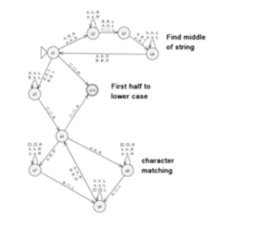
fig 3: combining turing machine

 • Copy TM

• See in action

●      Useful "subroutines"

-         Something to be noted

●      The TM must be configured to be in the correct position. The configuration is "called" before delete.

●      I.e. the head of the tape must be at the sign to be Removed.

6.4 Computing partial function with a TM

Being a partial function, a TM transition feature means that there are input pairs for which the transition feature is not defined.

δ (non-halting-state, symbol) = UNDEF

By adding a new dedicated "run forever" state, R:, we can easily compensate for such an omission

δ(R,σ) = (R,σ) ∀ σ ∈ Σ

Simply send a missing transition to this state without tape modification with this addition, i.e.,

δ(non-halting-state, symbol) = (R, symbol)

The easiest computer we can create that runs indefinitely is this:

Run Forever = ( {s,h}, Σ, {}, s, {h} )

There are states of beginning and halt, but no transitions, implying that all transitions go to some state of "run forever"

6.5 Multi-tape TMs, and Universal TM

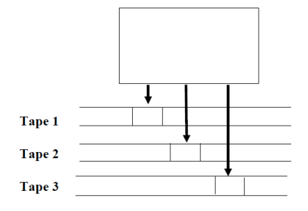
Multitape TM

fig 4: multitape TM

– Initially,

• the input string is placed on the 1st tape;

• the other tapes hold all blanks;

• the finite control is in its initial state;

• the head of the 1st tape is at the left end of the input;

• the tape heads of all other tapes are at arbitrary positions.

– A move consists of the following steps:

• the finite control enters a new state;

• on each tape, a symbol is written;

• each tape head moves left or right, or stationary.

Universal TM

A Turing Machine is the mathematical tool equivalent to a digital computer. It was

suggested by the mathematician Turing in the 30s, and has been since then the

most widely used model of computation in computability and complexity theory.

The model consists of an input output relation that the machine computes. The input

is given in binary form on the machine’s tape, and the output consists of the contents

of the tape when the machine halts.

What determines how the contents of the tape change is a finite state machine (or

FSM, also called a finite automaton) inside the Turing Machine. The FSM is

determined by the number of states it has, and the transitions between them.

At every step, the current state and the character read on the tape determine the

next state the FSM will be in, the character that the machine will output on the tape

(possibly the one read, leaving the contents unchanged), and which direction the

head moves in, left or right.

The problem with Turing Machines is that a different one must be constructed for

every new computation to be performed, for every input output relation.

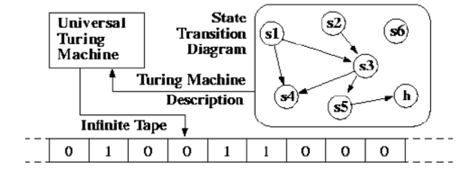
This is why we introduce the notion of a universal turing machine (UTM), which

along with the input on the tape, takes in the description of a machine M. The UTM

can go on then to simulate M on the rest of the contents of the input tape.

 A universal turing machine can thus simulate any other machine.

Fig 5: universal turing machine

Key takeaway:

●      A Turing Machine is the mathematical tool equivalent to a digital computer.

●      The model consists of an input output relation that the machine computes.

●      A universal turing machine can thus simulate any other machine.

References:

1. John E. Hopcroft, Rajeev Motwani and Jeffrey D. Ullman, Introduction to Automata Theory, Languages, and Computation, Pearson Education Asia.
2. Michael Sipser, Introduction to the Theory of Computation, PWS Publishing.
3. John Martin, Introduction to Languages and the Theory of Computation, Tata McGraw Hill.