UNIT 4
DYNAMIC PROGRAMING
• Dynamic programing solves the solutions of sub-problems
• Dynamic programing applies when sub-problem overlaps
• It solves each sub-problem just ones and then saves answer in table.
• Dynamic programing follows the basic principle of optimality.
• The principle of optimality says that problem can solve by taking some decisions.
• In greedy method we take decisions at one time only but in dynamic we take decisions at every stage.
• Binary search tree is the rooted binary tree which is divided into sub-trees.
• Left node having lesser value than root and right node having the greater value than root.
• Optimal binary search tree is the tree with the minimum cost value.
Suppse we have inputs as keys and frequency.
Input [10,20,30]
Freq [3,2,5]
Following are the possibilities:
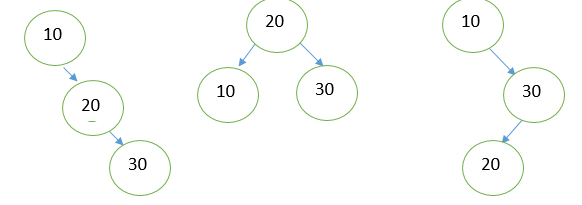
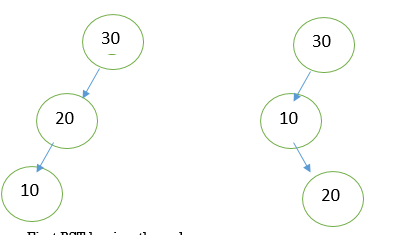
First BST having the value:
10----------------1*3=3
\ min value of BST is : 3+4+15=22
20------------2*2=4
\
30----------3*5=15
II= 20 III= 10 IV=30 V= 30
/ \ \ / /
10 30 30 20 10
/ / \
20 10 20
19 18 17 18
So among all BSTs, IV th BST has optimal solution as 17 is minimum cost value of binary tree.
• 0/1 knapsack problem is used to find the maximum profit from the items selected.
• 0/1 knapsack problem means we pick the item or not picking the item ie. We canot split the item.
• Item having the weight and the cost.
• Assume we are having many item then which item will give us profit more than we have ti check first.
• First sort the value to weight in non-increasing order and then pick the item.
Here I is row and j is column
If (j<wt[i])
T[i][j]=T[i-1][j]
Else
{
T[i][j]=max{val[i]+T[i-1][j-wt[i]]
or
{T[i-1][j]
Here total weight =7
value | weight | 0 | 1 | 2 | 3 | 4 | 5 | 6 | 7 |
1 | 1 | 0 | 1 | 1 | 1 | 1 | 1 | 1 | 1 |
4 | 3 | 0 | 1 | 1 | 4 | 5 | 5 | 5 | 5 |
5 | 4 | 0 | 1 | 1 | 4 | 5 | 6 | 6 | 9 |
7 | 5 | 0 | 1 | 1 | 4 | 5 | 7 | 8 | 9 |
• In travelling salesman problem start with source node travel all the nodes once and come back to the starting node and which path gives the minimum cost for travelling that becomes the optimal solution for travelling salesman problem.
• Formula:
G(i,s)=min{Cik+ G( k, S- { k } )}
Example:
| 1 | 2 | 3 | 4 |
1 | 0 | 10 | 15 | 20 |
2 | 5 | 0 | 9 | 10 |
3 | 6 | 13 | 0 | 12 |
4 | 8 | 8 | 9 | 0 |
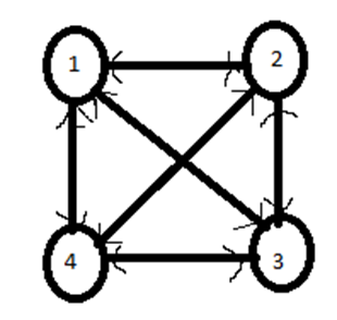
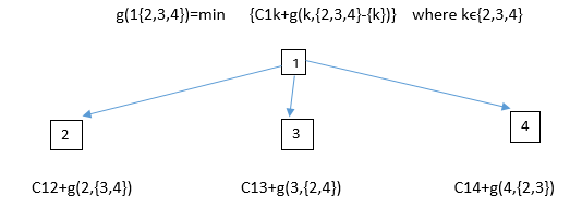
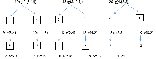
13+5=18
G(2.ф)=5
G(3.ф)=6
G(4.ф)=8
G(2,{3})=15
G(2,{4})=18
G(3,{2})=18
G(3,{4})=20
G(4,{2})=13
G(4,{3})=15
G(2,{3,4})=25
G(3,{2,4})=25
G(4,{2,3})=23
G(1,{2,3,4})=35
So the minimum optimal cost value from source node 1 to all other node is 35.
• Floyds algorithm is used to find shortest path from one node to all other nodes in the network.
• Hence it is also known as all pair shorteset path algorithm.
• Suppose there are four nodes such as A,B,C,D. If source node is A then it finds the shortest path from A to all other nodes in network as shown in figure given below.
Example:
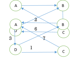
Step1: construction of matrix D0
If i=3 then Wij=’--’
Else if ij={C}
Else mark ∞
D0=
| a | b | c | D |
A | - | ∞ | 3 | ∞ |
B | 2 | - | ∞ | ∞ |
C | ∞ | 7 | - | 1 |
D | 6 | ∞ | ∞ | - |
Step 2:
Wij k = min(Wij k-1,Wik k-1+ Wkj k-1)
| a | b | c | D |
A | - | ∞ | 3 | ∞ |
B | 2 | - | 5 | ∞ |
C | ∞ | 7 | - | 1 |
D | 6 | ∞ | 9 | - |
D1 =
Step 3:
| a | b | c | D |
A | - | ∞ | 3 | ∞ |
B | 2 | - | 5 | ∞ |
C | 9 | 7 | - | 1 |
D | 6 | ∞ | 9 | - |
D2=
Step 4:
| a | b | c | D |
A | - | 10 | 3 | 4 |
B | 2 | - | 5 | 6 |
C | 9 | 7 | - | 1 |
D | 6 | 16 | 9 | - |
D3=
| a | b | c | D |
A | - | 10 | 3 | 4 |
B | 2 | - | 5 | 6 |
C | 7 | 7 | - | 1 |
D | 6 | 16 | 9 | - |
D4=
D4 is the final matrix where we remove all the ∞ value and now each node having shortest distance from each other.
This graph is directed graph where G=(V,E) is directed graph.
In this vertices are partitioned into k where k>1 number of disjoint subset S={s1,s2,……,sn} such that edge (u,v) is in E, then uϵS and VϵS for some subsets in the partition and |s1| = |sk| = 1.
The vertex s Є s1 is called the source and the vertex t Єsk is called sink.
G is usually assumed to be a weighted graph.
In this graph, cost of an edge (i, j) is represented by c(i, j).
Hence, the cost of path from source s to sink t is the sum of costs of each edges in this path.
The multistage graph problem is finding the path with minimum cost from source s to sink t.
Example
Consider the following example to understand the concept of multistage graph.
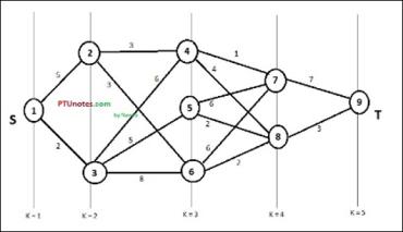
According to the formula, we have to calculate the cost (i, j) using the following steps
Step 1: Cost (K-2, j)
In this step, three nodes (node 4, 5. 6) are selected as j. Hence, we have three options to choose the minimum cost at this step.
Cost(3, 4) = min {c(4, 7) + Cost(7, 9),c(4, 8) + Cost(8, 9)} = 7
Cost(3, 5) = min {c(5, 7) + Cost(7, 9),c(5, 8) + Cost(8, 9)} = 5
Cost(3, 6) = min {c(6, 7) + Cost(7, 9),c(6, 8) + Cost(8, 9)} = 5
Step 2: Cost (K-3, j)
Two nodes are selected as j because at stage k - 3 = 2 there are two nodes, 2 and 3. So, the value i = 2 and j = 2 and 3.
Cost(2, 2) = min {c(2, 4) + Cost(4, 8) + Cost(8, 9),c(2, 6) +
Cost(6, 8) + Cost(8, 9)} = 8
Cost(2, 3) = {c(3, 4) + Cost(4, 8) + Cost(8, 9), c(3, 5) + Cost(5, 8)+ Cost(8, 9), c(3, 6) + Cost(6, 8) + Cost(8, 9)} = 10
Step 3: Cost (K-4, j)
Cost (1, 1) = {c(1, 2) + Cost(2, 6) + Cost(6, 8) + Cost(8, 9), c(1, 3) + Cost(3, 5) + Cost(5, 8) + Cost(8, 9))} = 12
c(1, 3) + Cost(3, 6) + Cost(6, 8 + Cost(8, 9))} = 13
Hence, the path having the minimum cost is 1→ 3→ 5→ 8→ 9.
This is a problem where several devices are connected in series.

Let assume that reliability device is r1 then its reliability function is πr1.
If r1 = 0.99 and n = 10 that n devices are set in a series, 1 <= i<= 10, then reliability of the whole system πri can be given as: Πri = 0.904
So, if we duplicate the devices at each stage then the reliability of the system can be increased.
It can be said that multiple copies of the same device type are connected in parallel through the use of switching circuits.
Here, switching circuit determines which devices in any given group are functioning properly.
Then they make use of such devices at each stage, that result is increase in reliability at each stage.
If at each stage, there are mi similar types of devices Di, then the probability that all mi have a malfunction is (1 - ri)^mi, which is very less.
And the reliability of the stage I becomes (1 – (1 - ri) ^mi).
Thus, if ri = 0.99 and mi = 2, then the stage reliability becomes 0.9999 which is almost equal to 1.
Which is much better than that of the previous case or we can say the reliability is little less than 1 - (1 - ri) ^mi because of less reliability of switching circuits.
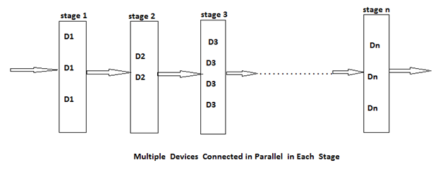
In reliability design, we try to use device duplication to maximize reliability. But this maximization should be considered along with the cost.