Unit 5
Curves and Surfaces
A curve is an infinite large set of points.
Each point has two neighbors except endpoints.
The classification of the curve is as follows:
The non-parametric curves can be explicit or implicit.
In non-parametric curves the y and z point on the curve are represented as two separate functions of the third coordinate x as the independent variable.
The curve which are having the parametric for then it is known as parametric curve.
The parametric curve is used for the practice purpose.
The representation of parametric curve in two dimensional form is,
P(t)=f(t) , g(t)
Or p(t)=xt,yt
The function f anf g become the x,y coordinates of any point on the curve.
The parameter t is varied over a certain interval (a,b), normally(0,1) then point is obtained.
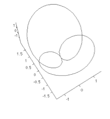
The space curves is a curve which lies in any region of three dimensional space.
It contrasted to aplane curve which must lie on single plane.
Space curve is very general form of curve.
The generation of the space curve is a problem of curve fitting for given set of points.
The approximation of curve for these data points is in space curve.
Following figure shows the representation of space curve.
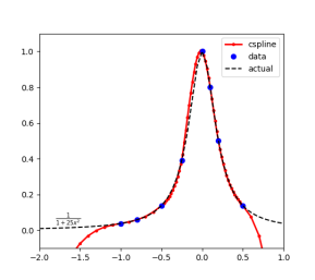
This spline constructed by piece pf third order polynomials.
This polynomial passes through set of m control points.
The polynomial’s second derivative is always set to be zero at endpoint which shows the boundary condition with system m-2 equation.
This spline is called as natural cubic spline.
Following figure shows the representation of cubic spline.
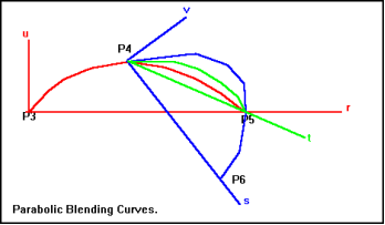
Let consider set of points p1,p2,p3….pn to interpolate a smooth curve.
Consider a section part p3,p4,p5,p6 where assume one parabola (Pr) is fitted in p3,p4,p5 and second parabola (Qs) to the points p4,p5,p6.
For interval at p4,p5 the parabola is overlap where we can blend them to make a smooth curve from p4 to p5.
The representation of first parabola is given in coordinates (r, u) with the origin at the point p3.
R is measured along line p3p5 and u is perpendicular to r.
Hence equation of u become,
U=P(r)=K1 * r * (r2-r)
K1 is the value of curve that passes through point p4.
The second parabola is also calculated same as first parabola.
V=Q(s)= K2 * s * (s2-s)
K2 is value of curve passes from point p5
S1 is the value at point p5 and s2 at p6
V is perpendicular to v
The final quation that blens the curve from p4 to p5 is given as,
C(t)= [1 - t / t1] * P(r) + [t/t1] * Q(s)
Where, value takes from 0 at p4 and t1 at p5
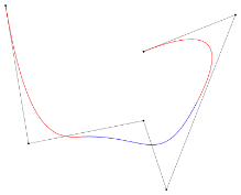
B-spline curve overcomes the limitation of Bezier curve as Bezier curve has limited flexibility.
It is a special case of Berstein basis.
It is non-global method.
It consists of linar combination of control points Pi and B-spline basis function Ni.
The mathematical representation of B-spline curve is,
C(t) = ∑ Pi * N(i,k)(t)
Where summation limitation is n to i=0 and n >= k-1, t belongs to (tk - 1, tn + 1)
Here k is order of polynomial seg,ents of B-spline curve.
N(i,k)(t) it is an normalized B-spline blending function.
Properties of B-spline curve:
The Bezier curve are developed by French engineer Pierre Bezier.
The Bezier curve is generated under the control of other points.
To generate the Bezier curve approximate tangents are used by using control points.
The mathematical representation of Bezier curve is,
∑ Pi * B ni (t) where summation from n to k=0
Pi is the set of points and B(t) is berstein polynomials as B(t)= (n , i)(1 - t)n-I * ti
The simple beizer curve is a straight line from P0 to P1.
A quadratic Bezier curve has three control points.
A cubic Bezier curve is determined by four control points.

Properties of Bezier curve:
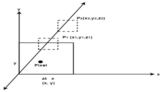
It is also called as Z – buffer algorithm.
It is a simplest image space algorithm.
The depth of object is computed by each pixel of the object displayed on the screen from this we get to know about how object closer to the observer.
The record of intensity is also keep with the depth that should be displayed to show the object.
It is an extension of frame buffer.
Two arrays are used for intensity and the depth, the array is indexed by pixel coordinates (x,y).
Algorithm:
Initially set depth(x,y) as (1,0) and intensity (x,y) to background value.
Find all the pixels (x,y) that lies on the boundaries of polygon when projected onto the screen.
To calculate pixel coordinates:
Calculate the depth z of the polygon at (x,y).
If z < depth (x,y) then this polygon lies closer to the observer else others are already recoreded for this pixel.
Set depth (x,y) to z and intensity(x,y) to the value according to polygon shading.
If z > depth (x,y) then this polygon is new and no action taken.
After all polygons have been processed the intensity array will contain the solution.
This algorithm contains common features to the hidden surface algorithm.
It requires the representation of all opaque surface in scene polygon in the given figure below.
These polygons may be faces of polyhedral recorded in the model of scene.
It is developed by John Warnock hence it is referred as Warnock algorithm.
In this the working of divide and conquer is applied.
The fundamental area of coherence is used.
The visibility of algorithm can be resolved by this algorithm.
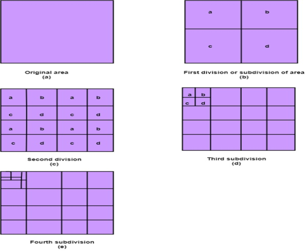
The classification of polygon takes place as trivial polygon and non-trivial polygon.
The trivial polygons are easy to handle.
The non-trivial polygons are divided into 4 equal sub windows then further division takes place until it becomes the trivial polygon.
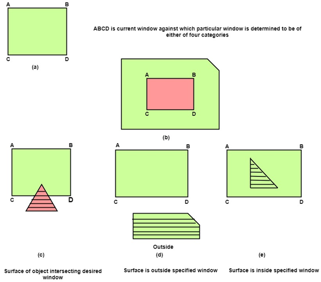
Following figure shows the classification of polygon takes place as trivial polygon and non-trivial polygon.
Following are four categories of polygons in Warnock algorithm:
Inside Surface: The surface that comes completely inside the boundaries or surrounding window.
Outside Surface: The surface that comes completely outside the boundaries or surrounding window.
Overlapping Surface: The surface that completely encloses the polygon surface or the surface that partially inside or outside the surface area.
Following figure shows the four categories of polygons in Warnock algorithm:
