Unit - 1
Introduction to Economics
Life is a never-ending sequence of decisions, some very complex and others relatively simple. Because we cannot know the future, we strive to reduce uncertainty in any decision by collecting as much information as possible. We designed this chapter to help you learn a logical decision-making process.
What is decision making?
Economic decision making is the process of making business decisions involving money. The purpose of making these decisions is generally to come up with strategies that help to either make the company more valuable or to increase the owner's revenue. Those involved in the decision-making process must have access to the company's detailed financial reports and must have a good understanding of the company's economic climate.
Success in the world of business depends on a company's leader ability to make wise economic decisions. Since economic decisions have to do with the amount of money a business earns or is valued at, it is essential that the decision-making process relies heavily on the company's financial reports. The outcome of the decisions being made should involve some type of monetary reward, and the decision-makers generally expect the reward to be much greater than the cost or sacrifice that's required to obtain it.
Financial decisions that benefit an organization often involve spending money. This money is often used to expand marketing strategies, recruit talent, increase production, improve product quality, and more. Financial decisions can also include the dismissal of an employee, the discontinuation of a particular product, the sale of a drink from a business, or the acquisition of a loan from a financial institution.
Key takeaways:
Business economics is actually part of economics and can simply be seen as a combination of economic theory and related theories related to business management. Business economics is a study that focuses on how economic theory affects the performance of real business or business activities. There are many practical case studies that have used economic theory for corporate development. For example, Product Lifecycle Theory described the entire Product Lifecycle from an economic perspective. It can be categorized by introduction, growth, maturity, and decline. Apple Inc. is a multinational technology company focused on electronic product design and development, and software development. The iPhone is one of the competitive advantages that brings huge profits to the company. However, as smartphone products are transitioning from maturity to decline, the competitive environment in the smartphone market is becoming fierce and profit margins are declining, so we are also considering research and development of new products such as electric vehicles as the competitive environment in smartphone market becomes fierce and profit margin has declined. The example has well explained the scenario where economic theories do help to support the decision-making in the practical business organisation.
What is Engineering Economics?
Engineering is the profession of applying mathematical and natural science knowledge gained through research experience and practice to judgments to develop ways to economically utilize natural materials and powers for the benefit of mankind.
Engineering economics is a very important theme for engineers. This subject helps to understand the need for knowledge of economics to become an effective manager and decision maker. The Economics theories are used to take decisions related to uncertain and changing business environment. Engineering economics quantifies the benefits and costs associated with engineering projects to determine if they can save enough money to justify capital investment. Engineering economics needs to apply the principles of engineering design and analysis in order to provide products and services that satisfy consumers at an affordable cost.
Special Characteristics:
Difference between Business Economy and Engineering
Economy is a social science that explains the factors that determine the production, distribution, and consumption of goods and services. Engineering economics is a subset of economics for application to engineering projects. Engineers seek solutions to problems, and the economic feasibility of each potential solution is usually considered along with the technical aspects. The engineering economy includes formulating, estimating, and assessing economic outcomes when alternatives are available to achieve defined objectives.
Key takeaways:
Demand is the percentage of consumers who want to buy a product. In Economic theory, we believe that demand is made up of two components: taste and purchasing ability. Taste, it's the desire for a good determines the willingness to buy the good at a particular price. Purchasing ability means that an individual must have sufficient ownership in order to purchase an item at a particular price.
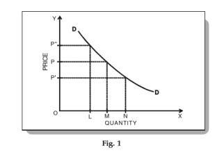
Both factors of demand depend on the market price. When the market price for a product is high, the demand will be low. When price is low, demand is high. At very low prices, many consumers will be able to purchase a product.
Supply
Willingness and ability to supply goods determine the seller’s actions. At higher prices, more of the commodity will be available to the buyers. This is because the suppliers will be able to maintain a profit despite the higher costs of production that may result from short-term expansion of their capacity.
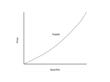
In a real market, when the inventory is less than the desired inventory, manufacturers will raise both the supply of their product and its price. The short-term increase in supply causes manufacturing costs to rise, leading to a further increase in price. The price change in turn increases the desired rate of production. A similar effect occurs if inventory is too high.
Key takeaways:
Demand analysis is the process by which management makes decisions regarding production, cost allocation, advertising, inventory holding, and pricing. The amount an enterprise produces depends on its production capacity, but depends on how much it has to strive for production.
Thus, the marketer is required to analyze properly the demand for its product in the market and must hold inventory accordingly. Such as if there is a potential demand in the future, then the firm should hold more inventories and in case there is no demand, then the production remains unwarranted, and hence, lesser inventories are held.
There is a possibility that production might exceed the demand, then the marketer must use alternative ways such as better advertisements to create a new demand. The demand shows the relationship between two economic variables, the price of the product and the quantity of product that a consumer is willing to buy for a given period of time, other things being equal.
Characteristics of Demand:
The following are the main characteristics or characteristics of the demand that the marketer must take into account when analyzing the demand for his product:
Key takeaways:
The elasticity of demand is an important variation on the concept of demand. You can classify the demand as Elastic, inelastic, or as single.
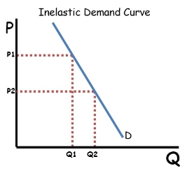
The elasticity of demand is the change in the quantity required due to price changes big. An inelastic demand is one in which the change in quantity demanded due to a change in the price is small.
The formula used here for computing elasticity of demand is:
(Q1 – Q2) / (Q1 + Q2)/ (P1 – P2) / (P1 + P2)
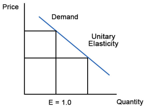
If the formula creates an absolute value greater than 1, the demand is elastic. In other words, quantity changes faster than price. If the value is less than 1, demand is inelastic. In other words, quantity changes slower than price. If the number is equal to 1, elasticity of demand is unitary.
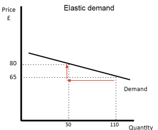
Elasticity of demand is illustrated in Figure 1. Note that a change in price results in a large change in quantity demanded. An example of products with an elastic demand is consumer durables. These are items that are purchased infrequently, like a washing machine or an automobile, and can be postponed if price rises. For example, automobile rebates have been very successful in increasing automobile sales by reducing price.
Close substitutes for a product affect the elasticity of demand. If another product can easily be substituted for your product, consumers will quickly switch to the other product if the price of your product rises or the price of the other product declines. For example, beef, pork and poultry are all meat products. The declining price of poultry in recent years has caused the consumption of poultry to increase, at the expense of beef and pork. So, products with close substitutes tend to have elastic demand.
Inelastic Demand
In figure 2 note that change in price results in only a small change in required quantity. In other words, the amount respondent is not very sensitive to changes in price. Examples of these are necessities like food. and fuel. Consumers will not cut down on their food shop if food prices go up, even though changes in the types of food they buy. Also, consumers will not change the way they drive much behaviour if gasoline prices rise.
Unitary Elasticity
If the elasticity coefficient is equal to one, demand is unitarily elastic as shown in Figure 3. For example, a 10% quantity change divided by a 10% price change is one. This means that a 1% change in quantity occurs for every 1% change in price.
Key takeaways:
What is demand forecasting?
Demand forecasting is the process of estimating future customer demand for a defined period of time using historical data and other information.
Good demand forecasting gives companies valuable information about their current and other market potential, allowing managers to make informed decisions about pricing, business growth strategies, and market potential.
Why is demand forecasting important?
There are a number of reasons why demand forecasting is an important process for business:
1. Sales forecasting helps with business planning, budgeting, and goal setting. Once you have a good understanding of what your future sales could look like, you can begin to develop an informed procurement strategy to make sure your supply matches customer demand.
2. It allows businesses to more effectively optimize inventory increase inventory turnover rates and reduce holding costs.
3. It provides an insight into upcoming cash flow, meaning businesses can more accurately budget to pay suppliers and other operational costs, and invest in the growth of the business.
4. Through sales forecasting, you can also identify and rectify any kinks in the sales pipeline ahead of time to ensure your business performance remains robust throughout the entire period. When it comes to inventory management, most eCommerce business owners know all too well that too little or too much inventory can be detrimental to operations.
Types of demand forecasting
Most traditional demand forecasting techniques fall into one of three basic categories:
Qualitative forecasting techniques are used when there is little data available, such as in a relatively new business or when a product is brought to market. In this case, use expert opinion, market research, comparative analysis, and other information to make a quantitative estimate of your demand.
This approach is often used in areas like technology, where new products may be unprecedented, and customer interest is difficult to gauge ahead of time.
2. Time series analysis
When historical data for a product or product line is available and trends are clear, companies tend to use a time series analysis approach to forecast demand. Time series analysis helps identify seasonal fluctuations in demand, cyclical patterns, and key sales trends.
The time series analysis approach is most effectively used by well-established businesses who have several years’ worth of data to work from and relatively stable trend patterns.
3. Causal models
Causal models are the most sophisticated and complex forecasting tools for businesses because they use specific information about the relationships between variables that affect market demand, such as competitors, economic strength, and other socio-economic factors. Like time series analysis, historical data is the key to making predictions for causal models.
For example, an ice cream business could create a causal model forecast by looking at factors such as their historical sales data, marketing budget, promotional activities, any new ice cream stores in their area, their competitors’ prices, the weather, overall demand for ice cream in their area, and even their local unemployment rate.
Key takeaways:
In ordinary language, the supply of a good means the quantity of the good that is available for sale in the market. Although a good is supplied in the market through the distributors, wholesalers, retailers and many other agencies, the ultimate supplier of a good is the firm that produces it, and it is assumed that the quantity supplied of a good per period is the same as the quantity produced of it per period.
Supply of a good in economics means the quantity produced and supplied of the good per period by its producer-firm(s) at any particular price of the good. However, supply depends on many things other than the price of the good.
For example, supply may depend on the cost of production of the good, the size and method of production, the business organisation of the firms producing it, the nature of the good, i.e., its perishability and lumpiness, the length of time obtained for effecting changes in the quantity produced, etc.
Individual Supply and the Law of Supply:
Traditional economic theory assumes that at a particular price of a good, an individual company / producer of the good produces / supplies an amount that maximizes his profits. This particular production, known as the equilibrium output of a company, is the individual supply of the company at the above prices.
Now, the curve that gives us an individual firm’s supply of a good at any particular price is called an individual supply curve for the good.
If the price of the good increases or decreases, an individual firm’s supply of the good would, generally, also increase or decrease. This is known as the law of supply. Owing to this law, an individual supply curve would generally slope upward towards right or would be positively sloped like the curves SS shown in Fig.
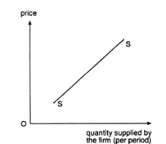
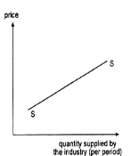
Fig. Supply Curve of an Individual Firm Fig. Supply Curve of Industry
Key takeaways:
Supply elasticity establishes a quantitative relationship between the supply of goods and their prices. Therefore, the concept of elasticity can be used to represent the numerical changes in supply as the price of goods changes. Note that elasticity can also be calculated for other supply determinants.
The price elasticity of supply is the ratio of the percentage change in the price to the percentage change in quantity supplied of a commodity.
Es= [(Δq/q) ×100] ÷ [(Δp/p) ×100] = (Δq/q) ÷ (Δp/p)
Δq= The change in quantity supplied
q= The quantity supplied
Δp= The change in price
p= The price
Elasticity from a Supply Curve
Along with the method mentioned above, there are two more ways to calculate the price elasticity of supply, both of which make use of the supply curve. We can either calculate the elasticity at a specific point on the supply curve, known as point elasticity or between two prices, known as arc-elasticity.
The formula for calculating the point elasticity of supply is:
Es= (dq/dp) ×(p/q)
Here dq/dp is the slope of the supply curve.
The formula for calculating the arc-elasticity of supply is:
Es= [(q1 – q2)/ (q1 + q2)] × [(p1 + p2)/ (p1 – p2)]
Types of Elasticity of supply
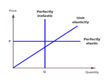
A service or goods, whatever the price, will be a completely inelastic supply if a certain quantity can be supplied. The elasticity of the supply of such services and goods is zero. A completely inelastic supply curve is a straight line parallel to the Y axis. This represents the fact that supply remains the same regardless of price.
2. Unitary Elastic
For a product with unit elasticity of supply, the change in the supply of the product is exactly the same as the change in its price. In other words, changes in both the price and supply of goods are proportional and equal to each other. To point out, the elasticity of the supply in such cases is equal to 1. In addition, a single elastic supply curve passes through the origin.
3. Perfectly Elastic demand
A commodity with a perfectly elastic supply has an infinite elasticity. In such a case the supply becomes zero with even a slight fall in the price and becomes infinite with a slight rise in price. This is indicative of the fact that the suppliers of such a commodity are willing to supply any quantity of the commodity at a higher price. A perfectly elastic supply curve is a straight line parallel to the X-axis.
Key takeaways:
We have studied demand and supply separately. Now we put them together to get the whole market. The operation of demand and supply in a market is known as the market mechanism.
We are familiar with the upward sloping supply curve and the downward sloping demand curve. Combine the two on one diagram and we have a model of market.
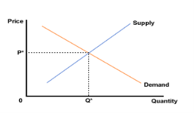
The market will be in equilibrium at price P, when quantity Q will be bought and sold. In figure 1 OP* is the equilibrium or market clearing price at which the amount demanded exactly matches the amount supplied.
Key takeaways:
References:
1. “Modern Micro Economics”, Koutsoyiannis.
2. “Fundamentals of Engineering Economics”, Park, Prentice Hall.
3. “Economics”, Samuelson.
4. “Growth Economics”, Sen A.K, Penguin Books, England.