Unit – 3
Production Function
To have clear knowledge about production and cost it’s mandatory to know the basics of production functions and understand the fundamentals in mathematical terms. We break down short-term and long-term production functions supported variable and glued factors.
What is the production function?
The functional relationship between the physical input (or factor of production) and therefore the output is named a production function. It assumed the input as an explanatory or independent variable and the output as a dependent variable. Mathematically, you can write this as:
Q=f (L, K)
Where "Q" represents the output, "L"and"K" are the inputs, respectively, labour and capital (such as machinery). Note that there may be many other factors, but we are assuming a two-factor input here. Production functions are defined differently in the short term and in the long term. This distinction is crucial in microeconomics. This distinction is based on the nature of the factor input.
Inputs that change directly with the output are called variable factors. These are factors that can change. Fluctuating factors exist both in the short term and in the long term. Examples of variable factors include daily labour and raw materials.
On the other hand, factors that cannot change or change as the output changes are called fixed factors. These factors are usually characteristic only for a short or short period of time. There are no fixed factors in the long term.
Therefore, two production functions can be defined: short-term and long-term. A short-term production function defines the connection between one variable factor (keeping all other factors fixed) and therefore the output. The law of regression to factors explains such a production function.
For example, suppose that a company has 20 units of Labour and 6 acres of land, and initially uses only Labour units (variable coefficients) for that land (fixed coefficients). Thus, the ratio of land and labour is 6: 1. Now, if the company chooses to adopt 2 labour units, then the ratio of land to Labour will be 3: 1 (6: 2).
Here, all factors change in the same proportion. The law used to explain this is called the law of return to scale. It measures how much of the output changes when the input changes proportionally.
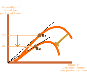
Fig 1. Production Function
Cobb-Douglas Production function
The Cobb-Douglas production function models the connection between production output and production input (factor). It is used to calculate the ratio of inputs to each other for efficient production and to estimate technological changes in production methods. The general form of the Cobb Douglas production function for a set of n inputs is: Y represents the output, xi represents the input i, and γ and αi are parameters that determine the overall efficiency of production and the responsiveness of the output to changes in input volume. The application of this functional form in the measurement of production was made by mathematician Charles Cobb and economist Paul Douglas from 1899 to 1922. In the original model, Cobb and Douglas ranged the output elastic parameters α1 and α2 αi ∈ Limit to (0,1) and limit the total to 1. This means a harvest on a certain scale. So, the function looks like this:
Y=f (x1, x2,..., xn)=γ∏i=1nxαii
Where x1 and x2 represent labor and capital, respectively. Taking the natural logarithms of each side of the equation gives:
Y=γxα11x1−α12
For data on production, workforce, and capital, the parameters γ and α1 can usually be estimated using the least squares method. Based on their data, Cobb and Douglas found that the value of α1 was 0.75. This means that the workforce accounted for three-quarters of US manufacturing output during the study. The estimated efficiency parameter γ is 1.01, which is greater than 1, reflecting the unobservable positive effect of force on production by the combination of labor and capital.
The multiplicative nature of the Cobb-Douglas production function means that the input is the complement of production, assuming the value of αi is positive. In the standard model of labor and capital, increasing the amount of capital increases production not only directly, but also indirectly through the impact on labor productivity. Mathematically, the partial derivative of production Y for labor x1 and capital x2 is positive. Furthermore, by assuming αi ∈ (0,1), the second partial derivatives of production and production with respect to labor and capital are both negative, meaning diminishing returns for each input only. Simply adding either labor or capital (but not both) to the production process will increase production but slow it down. In addition, the elasticity of the permutation between inputs is constant and equal to 1 due to the functional form. The two-input Cobb Douglas production function can be represented graphically in the form of an isoquant curve. That is, a combination of both inputs that have a constant output. The graph here has four isoquant curves with (constant) output levels Y1¯¯¯¯¯, Y2¯¯¯¯¯, Y3¯¯¯¯¯, and Y4¯¯¯¯¯. The farther the isoquant curve is from the origin, the higher the level of output. Y4¯¯¯¯¯> Y3¯¯¯¯¯> Y2¯¯¯¯¯> Y1¯¯¯¯¯. Which exact combination of inputs x1 and x2 is best for production depends on the budget available to the producer and the cost ratio of inputs x2 and inputs x1 that can be included in the graph in the form of cost-effective lines (See). Articles on alternative elasticity).
lnY=lnγ+α1lnx1+(1−α1)lnx2
Cobb and Douglas himself acknowledged that their production function was not based on a solid theoretical foundation and should not be understood as a law of production. It only represents a statistical approximation of the observed relationship between the inputs and outputs of production. Nevertheless, its simple mathematical properties are attractive to economists and have been the standard in microeconomic theory for the past century.
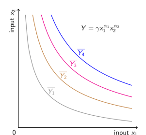
Fig 2. Cobb-Douglas Production Function
The Cobb-Douglas function form isn't only utilized in production theory, but also standardized in microeconomic consumer theory applied as a utility function, where Y is utility U. Next, xi represents the consumable item, and when the utility function is maximized according to the budget constraint, the value of αi indicates how the individual optimally allocates the budget among the items.
Economies of Scale
Economies of scale are defined as cost advantages that an organization can achieve by expanding its production over the long term.
In other words, these are the benefits of large-scale production of the organization. Cost benefits are achieved in the form of a low average cost per unit.
It's a long-term concept. Economies of scale are achieved when the turnover of the organization increases. As a result, the savings of the organization will increase, and it will be even more possible for the organization to obtain large amounts of raw materials. This will help the organization to enjoy discounts. These benefits are called economies of scale.
Economies of scale are divided into internal and external economies, which are discussed as follows:
i.Internal economy:
See the real economy arising from the expansion of the plant size of the organization. These economies arise from the expansion of the organization itself.
An example of an economy of internal size is:
a.Technical economy of scale:
It occurs when an organization invests in expensive and advanced technologies. This helps to reduce and control the production costs of the organization. These economies are enjoyed due to the technical efficiency obtained by the organization. Advanced technology allows organizations to produce a large number of goods in a short time. Thus, the industry-wide economy falls per unit of production costs
b.Marketing economy of scale:
Scale marketing economy is achieved in case of bulk purchase, branding, and advertising when large organizations have broadened their marketing budgets over large output. For example, large organizations enjoy the benefits of advertising costs as they cover a larger audience. On the other hand, small organizations pay the same advertising costs as big ones, but do not enjoy such benefits in advertising costs.
c.Financial economy of scale:
This happens when large organizations borrow money at a lower rate of interest. These organizations have good credibility in the market. In general, banks prefer to grant loans to organizations that have a strong foothold in the market and have good repayment capacity.
d.Management economy of scale:
During the occurrence of large organizations specialized workers for different things. These workers are experts in their respective fields and use their knowledge and experience to maximize the benefits of the organization. For example, in an organization, accounts and research departments are created and managed by experienced individuals so that all costs and benefits of the organization can be properly estimated.
E.Commercial economy:
See an economy where organizations enjoy the benefits of purchasing raw materials and selling finished products at a lower cost. Large organizations buy raw materials in bulk; therefore, enjoy the advantages of transportation charge from Bank, easy credit, and prompt delivery of products to customers.
ii.Foreign economy:
Occurs outside the organization. These economies arise within industries that benefit organizations. If the industry expands, the organization will benefit from better transport networks,infrastructure and other facilities. This will help reduce the cost of the organization.
Some examples of economies of external scale are discussed as follows:
A.Economy of concentration:
See the economy resulting from skilled labor, better credit, and the availability of transport facilities.
B.Economy of information:
Means the benefits gained from trade and business related publications. The central research institution is the source of information for the organization.
C.Collapsing economy:
Refer to the division of associations caused by the economic process into different processes.
Uneconomics of scale occurs when the long-term average cost of an organization increases. It can occur when the tissue becomes excessively large. In other words, uneconomics of Scale Causes larger org-anizations to produce goods and services at increased costs.
There are two types of scale diseconomies: internal diseconomies and external diseconomies, which are discussed as follows:
i.Internal uneconomics of the scale:
See uneconomical raising the cost of production in the organization. The main factors affecting the cost of production of the organization include the lack of determination, supervision and technical difficulties.
ii.External uneconomics of the scale:
See uneconomical to limit the expansion of an organization or industry. Factors acting as restraints on expansion include increased production costs, a shortage of raw materials and a decline in the supply of skilled workers.
There are several causes of diseconomics of scale.
Some of the causes that lead to uneconomics of scale are:
i.Act as the main reason for diseconomics of scale.
If the organization's production goals and objectives are not properly communicated to employees in the organization, they can lead to overproduction or production. This can lead to diseconomics of scale.
Separately, if the communication process in the organization is not strong, then the employee will not get enough feedback. As a result, there will be less face-to-face interaction between employees, which will affect the production process.
ii.Lack of motivation:
This leads to a decrease in productivity levels. For large organizations, workers may feel isolated and less motivated because they are less valued for their work. Because of poor communication networks, it is difficult for employers to interact with employees and build a sense of attributes. This leads to a decrease in the productivity level of output due to lack of motivation. This further leads to an increase in the cost of the organization.
iii.Loss of control:
It serves as the main problem of large organizations. Monitoring and controlling the work of all employees in a large organization becomes impossible and expensive. It is difficult to make sure that all employees of the organization are working towards the same goal. It becomes difficult for managers to direct the sub-coordinates of large organizations.
iv.Cannibalism:
It means a situation where an organization is facing competition from its products. While smaller organizations face competition from the products of other organizations, larger organizations find their products compete with each other.
Key takeaways:
Buyers and Sellers of Homogeneous Products.
The price of a product is determined by the industry by the forces of supply and demand. For example, if you need a pen, there should be several shops selling pens. Under the conditions of perfect competition, every seller must sell the same quality of the pen at a uniform prevailing price on the market. You can buy a pen from any store at the price Rs. 10. If another shopkeeper charged Rs. 12 for the same quality of the pen, nobody buys from him. But if the shopkeeper charged Rs. 9 all buy pens from that particular store. But both of these situations are unrealistic.
There must be one price dominant throughout the market. Therefore, full competition in the market structure is characterized by a complete lack of competition between individual companies.
Definition:
It is identified by the existence of the many firm; they all sell an identical products an equivalent way. The supplier is the one who accepts the price."- Vilas
Such market gains when the request for product of every producer is totally elastic. Mrs Joan Robinson.
It is a market condition with an outsized number of sellers and buyers, similar products, free entry of enterprises into the industry is ideal knowledge between buyers and sellers of existing market conditions and free mobility of production factors between alternative uses. Lim Chong-ya
Assumption:
The following assumptions for a fully competitive market:
1. A large number of buyers and sellers:
This affects single buyers and sales. When a company enters or leaves the market, there is no impact on the supply. Similarly, if a buyer enters or withdraws from the market, demand will not be affected. Such affects individual buyers and sellers.
2. Homogeneous products:
The second assumption of perfect competition is that all sellers sell homogeneous products. In this situation, the buyer has no reason to prefer the product of one seller to another. This condition exists only if the goods have a clear chemical and physical composition, that is, Substances of the specified grade: salt, tin, wheat, etc.
3. No discrimination:
Under complete competition in the market, sellers and buyers, sellers do freely. It means that buyers and sellers must be willing to deal openly with each other to buy and sell at market prices. This may be true of everything you might want to do so without offering special deals, discounts, or favours to selected individuals.
4. Perfect knowledge:
The competitive market is me (buyers and sellers are in close contact with each other. It means that, on the part of buyers and sellers, there is complete knowledge of the market. This means that many buyers and sellers in the market know exactly how much the price of the goods is in different parts of the market.
In other words, without the knowledge of each buyer and seller of the price at which the transaction is taking place, and the price at which the other buyer and seller are willing to buy or sell.
5. Industry FREE entry and exit:
In the long run, under full competition, the company can enter or exit the enterprise. There is no let or hindrance to the enterprise with regard to its entry into or exit from the market. In other words, the company has no legal or social restrictions. A large number of sellers is possible only if there is a free entry of the enterprise.
6. Perfect mobility:
There must be full mobility of domestic production factors that ensure uniform production costs throughout the economy. That means you are free to seek employment in any industry where different factors in production might like you.
7. Profit maximization:
Under perfect competition, all companies have a common goal of maximizing profits. Thus, there is a lack of social welfare of the general public.
8. No sales cost:
Under perfect competition, there is no sales cost.
9. No transportation costs:
Transportation costs between the sellers should not be. If transportation costs are present buyers are prevented from moving from one seller to another to take advantage of the price difference, which means that transportation costs do not affect the pricing of the product. In other words, these are always prices uniform in the market.
Pure and perfect competition:
Many economists choose to use the term "free market" rather than" pure competition.", American economists particularly prefer the term pure competition over the term perfect competition, but the term perfect competition seems to be popular with British economists.
But Professor Chamberlain distinguished between perfect competition and pure competition. Contains pure competition, according to Professor Chamberlain:
(I) numerous buyers and sellers,
(II) Homogeneous products,
(III) Free entry and exit of industry,
(IV) free from checks,
(V) lack of sales costs, and
(VI) lack of transportation costs.
R.A. Professor Bilas also distinguished between perfect competition and pure competition “perfect competition means pure competition, but we also consider other characteristics. Pure competition implies a certain degree of perfection, that is, the complete absence of monopoly.
In general, perfect competition leads to perfect resource mobility and perfect knowledge concepts. Similarly, professor Baumol defined pure competition as industry. Many companies are said to operate under pure competition when there is, product homogeneity, freedom of entry and exit, independent decision making.”
Based on these definitions, we can say that pure competition exists when an element of Monopoly is not present in the market. Perfect competition is wider than pure competition, including the absence of monopolies, as well as perfection in many other ways, such as full mobility of production factors and full knowledge of the market. Therefore, producers have complete knowledge of the quantity and quality of available production factors, as well as the prices that can be charged for their products.
Therefore, the distinction between pure competition and perfect competition is simply of a degree, and all assumptions of pure competition are also assumptions of perfect competition the concept of a complete competition system includes one more assumption: viz.Be perfect knowledge by both buyers and sellers of prevailing market prices, and different range and quality of various goods, services and production factors.
Imperfect Competition: Difference between perfect competitions, monopoly and imperfect competition
Given below can explain the major differences between the three markets
Perfect competition is a concept in microeconomics that describes a market structure that is completely controlled by market forces. If these forces are not met, the market is said to have incomplete competition.
There is no market that clearly defines full competition, but all real world markets are classed as incomplete. That is, perfect markets are used as a standard that can measure the effectiveness and efficiency of real world markets.
Perfect competition:
1. An outsized number of buyers and sellers.
2. Perfect competition among sellers.
3. Homogeneous products.
4. Lack of control over the factors of production.
5. Lack of price controls
6. Complete knowledge of the market.
7. One price or an equivalent price prevails everywhere.
Imperfect competition
Incomplete competition occurs in a market when one of the conditions of a fully competitive market is left unfulfilled. This type of market is very common. In fact, every industry has some type of incomplete competition. This includes various products and services, prices that are not set by supply and demand, competition for market share, buyers who do not have complete information about products and prices, and high barriers to entry and exit.
Incomplete competition is found in the following types of market structures: monopolies, oligopolies, monopolies, and oligopoly.
In monopolies, there is only one (dominant) seller. The company offers products to markets where there are no substitutes. Monopolies have high barriers to entry and there is a single seller who is a price maker. That means the company sets the price at which the product is sold regardless of supply or demand. Finally, the company can change the price at any time without notifying the consumer.
In oligopolies, there are many buyers, but only a few sellers. Oil companies, grocery stores, mobile phone companies, and tire manufacturers are examples of oligopolies. As there are few players dominating the market it may block others from entering the industry. Companies with this market structure can do so if they set prices for products and services in bulk or, in the case of cartels, take the lead.
Imperfect competition:
1. Little number of buyers and sellers.
2. Incomplete competition of sellers.
4. Artificial restrictions on production factors.
5. The presence of control.
6. Ignorance of purchase.
7. Price discrimination.
Monopoly:
1. Just one seller.
2. Lack of competition.
3. there's no product differentiation.
4. Artificial restrictions on production factors.
5. Full control of price.
6. Incomplete knowledge of the market.
7. Price discrimination.
Allocation efficiency under Perfect Competition
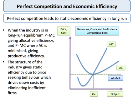
Fig. 3 Perfect Competition
In free market, market cost reflects the complete s of resources and freedom of entry and exit, full access to information by all participants, homogeneous products and therefore the incontrovertible fact that nobody buyer or seller, or a gaggle of buyers or sellers, has any advantage over others.
Perfect competition is often used as a measure to match with other market structures, because it displays a high level of economic efficiency. Allocation efficiency:
We can see that within the short and future, the worth is adequate to the incremental cost (P=MC) and thus the allocation efficiency is achieved.
The ruling price maximizes the excess of consumers and producers.
No one can make better without making other agents a minimum of as worse–i.e. we achieve Pareto optimum allocation of resources.
Production efficiency:
Production efficiency occurs when balanced output is supplied at a minimum monetary value. This is achieved within the future for a competitive market.
Companies with higher unit costs might not be ready to justify remaining within the industry as market prices are pushed down by the force of competition.
Dynamic efficiency:
That is, there's little scope for innovation designed purely to differentiate products and permit suppliers to develop competitive advantages within the market and establish monopoly power.
Perfect competition-the chain of reasoning
Is perfect competition good for economic efficiency?
Some economists believe that perfect competition isn't an honest market structure for top levels of research and development spending and therefore the resulting product and process innovation.
Indeed, monopolistic or oligopolistic markets could also be simpler within the end of the day in creating an environment for research and innovation to flourish. Cost-cutting innovation from one producer is completed immediately, assuming perfect information, without transferring costs to all or any other suppliers.
That said, a competitive market would offer discipline for companies to regulate costs, minimize waste of scarce resources, set high prices and refrain from exploiting consumers by enjoying high profit margins. During this sense, competition can stimulate improvements in static and dynamic efficiency over time.
The future of perfect competition therefore exhibits an optimal level of economic efficiency. However, for this to be achieved, all of the conditions of full competition, including the relevant market must hold.
Monopoly: Short-run and long-run equilibrium of monopoly firm
A. Short run
A monopolist maximizes his short-term profits if the following two conditions are met first, MC equals Mr. Secondly; the slope of MC is larger than that of Mr at the intersection.
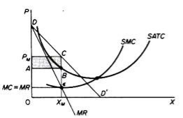
Fig.4 Equilibrium of The Monopoly
In Figure 4, the equilibrium of the monopoly is defined by the point θ at which MC intersects the MR curve from below. Thus, both conditions of equilibrium are met. The price is PM and the quantity is XM. Monopolies realize excess profits equal to shaded areas APM CB. Please note that the price is higher than Mr
In pure competition, the company is the one who receives the price, so its only decision is the output decision. The monopolist is faced with two decisions: to set his price and his output. But given the downward trend demand curve, the two decisions are interdependent.
Monopolies set their own prices and sell the amount the market takes on it, or produce an output defined by the intersection of MC and MR and are sold at the corresponding price. An important condition for maximizing the profits of monopolies is the equality of the MC and the MR, provided that the MC cuts the MR from below.

We can now revisit the statement that there is no unique supply curve for the monopolist derived from his MC. Given his MC, the same amount could be offered at different prices depending on the price elasticity of demand. This is graphically shown in Figure 5. Quantity X is sold at price P1 if demand is D1, and the same quantity X is sold at price P2 if demand is D2.
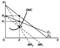
Fig 5. Price Elasticity of Demand
So, there is no inherent relationship between price and quantity. Similarly, given the monopolist MC, we can supply various quantities at any one price, depending on the market demand and the corresponding MR curve. Figure 6 illustrates this situation. The cost condition is represented by the MC curve. Given the cost of a monopolist, he would supply 0X1 if the market demand is D1, then p at the same price, and only 0X2 if the market demand is D2 B. Long-term equilibrium:
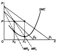
Fig. 6 Market Demand
In the long run the monopolist will have time to expand his plants or use his existing plants at every level to maximize his profits. However, if the entry is blocked, the monopolist does not need to reach the optimal scale (that is, the need to build the plant until the minimum point of LAC is reached), neither does the guarantee that he will use his existing plant at the optimum capacity. What is certain is that if he makes a loss in the long run, the monopolist will not stay in business.
He will probably continue to earn paranormal benefits even in the long run, given that entry is banned. But the size of his plant and the degree of utilization of any plant size depends entirely on the market demand. He may reach the optimal scale (the minimum point of Lac), stay on the less optimal scale (the falling part of his LAC), or exceed the optimal scale (expand beyond the minimum LAC), depending on market conditions.
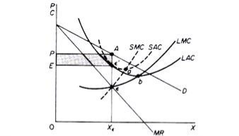
Fig. 7 Monopolist with suboptimal Plant and excess Capacity
Figure 7 shows when the market size does not allow the monopolist to expand to the minimum point of Lac. In this case, not only is his plant not optimal (in the sense that the economy of full size is not depleted), but also the existing plant is not fully utilized. This is because on the left of the minimum point of the LAC, the SRAC touches the LAC at its falling part, and the short-term MC must be equal to the LRMC. This happens in e, but the minimum LAC is b, and the optimal use of the existing plant is a. Since it is utilized at Level E', there is excess capacity. Finally, figure 8 shows a case where the market size is large enough for a monopolist to build an optimal plant and be able to use it at full capacity.
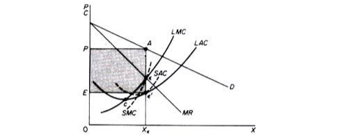
Fig. 8 Monopoly operating in a large market: his plant is larger than Optimal © and is being overutilized
In Figure 9, the scale of the market is so large that monopolists have to build plants larger than the optimal ones to maximize output and over-exploit them. This is because to the right of the minimum point of LAC, SRAC and LAC is tangent at the point of positive slope, and SRMC must be equal to LAC. Thus, plants that maximize the profits of monopolies are, firstly, larger than the optimal size, and secondly, they are over-utilized, which leads to higher costs. This is often the case with utility companies operating at the state level.
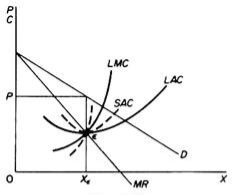
Fig 9. Scale of The Market
It should be clear that which of the above situations will appear in a particular case will depend on the size of the market (given the technology of monopolists). There is no certainty that monopolies will reach their optimal size in the long run, as is the case with purely competitive markets. In Monopoly, there is no market force similar to those of pure competition that will lead companies to operate at optimal plant size in the long run (and utilize it at its full capacity).
Concept of supply curve under monopoly
The supply curve under incomplete competition or Monopoly is not unique.
This is due to the fact that, unlike full competition, the price is determined simultaneously with the volume of goods produced, and the price is not given to the enterprise under monopoly or Monopoly competition.
Here the company is the price manufacturer of her products. Therefore, the company fixes the price at which it will get the maximum profit. The supply of goods is determined by the market demand for its products. Therefore, it is impossible to talk about the supply curve under monopoly or Monopoly competition.
The output supplied by the producer under such exclusive circumstances depends on the market demand conditions of his product and draws a unique supply curve (and supply schedule).
Therefore, it is not quite applicable to the causes of incomplete competition, monopoly competition, monopolies and oligopolies. This is because the concept of the supply curve refers to questions about the amount of goods a company supplies at various given prices.
Under various sorts of incomplete competition, individual companies don't take the worth as given and aren't mere quantity adjusters. In fact, under various forms of incomplete competition, the company sets its own prices. For companies under incomplete competition, it is not a matter of adjusting output or supply at a given price, but choosing a combination of price output that maximizes profit.
Commenting on the relevance of the supply curve, professor Baumol writes: the supply curve is, strictly speaking, a concept usually relevant only in the case of pure (or complete) competition...The reason for this lies in its definition—the supply curve is designed to answer the form question, “to answer the form question how much would solidify the supply if it encounters a price that is fixed in P dollars. But such questions are most relevant to the behavior of companies that actually deal with prices.”
Allocation inefficiency and dead-weight loss monopoly
Monopoly
Monopolies exist when a particular enterprise is the sole supplier of a particular commodity. Monopoly has little to no competition when producing good or service. Monopolies are entities that have significant market power (the power to charge high prices).
Inefficiency in Monopoly
In monopolies, the company sets a certain price for the goods that are available to all consumers. The quantity of good things will be less, and the price will be higher (this is what makes good things a commodity). Monopoly pricing creates a burden loss because companies forgo transactions with consumers. The burden loss is a potential gain that hasn't gone to producers or consumers. As a result of the loss of burden, the combined surplus (wealth) of monopolies and consumers is less than that obtained by consumers in competitive markets. Monopolies are less effective in total profits from trade than in competitive markets.
Monopolies can become inefficient and less innovative over time, because they do not have to compete with other producers in the market. For private monopolies, complacency can overcome barriers to entry and create room for potential competitors to enter the market. In addition, long-term alternatives in other markets can take control when monopolies become inefficient.
Market failure
If the market is unable to allocate resources efficiently, a market failure occurs. In the case of monopolies, abuse of power can cause market failure. Market failure occurs when the price mechanism does not take into account all of the costs and/or benefits of providing and consuming goods. As a result, the market is not able to supply socially optimal quantities of goods. Monopolies are imperfect markets that limit output in an attempt to maximize profit. Monopoly market failure can happen because enough of the great isn't made available and/or the worth of the great is just too high. Without the presence of competitors in the market it can be a challenge for monopolies to self-regulate and remain competitive over time.


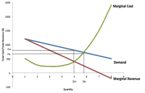
Fig. 10 Market failure
In economics, weight loss is a loss of economic efficiency that occurs when the equilibrium of goods or services is not Pareto optimal. If good or service is not the optimal Pareto, economic efficiency is not equilibrium. As a result, when resources are allocated, it is impossible to make any individual better, without worsening at least one person. When weight loss occurs, there is a loss in the economic surplus in the market. Weight loss means that the market cannot be cleared naturally.
Causes of loss of dead weight
The loss of a dead weight is the result of a market that cannot be cleared naturally and is therefore an indicator of market inefficiency. Supply and demand for goods or services are not balanced. The causes of weight loss are:
Dead Loss decision
To determine weight loss on the market, the formula P=MC is used. The loss of the dead weight is equal to the change in price multiplied by the change in the required quantity. This formula is used to identify the causes of inefficiencies in the market.
For example, in a nail market where the cost of each nail is$0.10, demand decreases from high demand for cheap nails to zero demand for nails at$1.10. In a fully competitive market, producers will charge$0.10 per nail, and every consumer whose marginal profit exceeds$0.10 will have a nail. But if one producer has a monopoly on nails, they charge a price that brings the maximum profit. If they charge$0.60 per nail, all parties that have less than$0.60 of marginal gains will be excluded. If equilibrium is not achieved, the parties that would have entered the market with pleasure are excluded for non-market prices.
Sometimes policymakers impose binding constraints on items if they believe that the benefits from the transfer of surpluses outweigh the negative effects of the loss of burdens.
Monopolistic Competition: Assumption
Years ago in 1920s, the classical theory of price included two main models: pure competition and monopoly.
The double occupancy model was considered an intellectual exercise, not a real-world situation. The general model of economic behavior from Marshall to Knight was pure competition.
In the late 1920s, economists became increasingly frustrated with the use of pure competition as an analytical model of business behavior. It was clear that pure competition could not explain some empirical facts.
Moreover, the practice of advertising and other sales activities can not explain the widely used businessman pure competition. Finally, as we predict when a pure competitive model will continuously reduce costs, companies have expanded their output with reduced costs, but never grow infinitely large.
In particular, it was this last fact of falling costs that created discontent and caused a widespread reaction to pure competition theory. This discontent caused a long series of debates and the publication of numerous articles that formed the"great cost controversy of the 1920s.
The earliest summary of the cost controversy should be found in Piero Sraffa's article. Sraffa pointed out that the falling cost dilemma of classical theory can be theoretically solved in various ways by introducing a demand drop curve for individual companies, a general equilibrium approach that appropriately incorporates the shift in costs induced by external economies (firms and industries), or by introducing a U-shaped sales cost curve into the model.
Of these solutions, Sraffa was the first to adopt, that is, a model with a negative personal demand curve that was more operationally and theoretically more plausible. The same line is a work published in 1933, in which E.It was adopted independently by Chamberlin and Joan Robinson.
It should be noted that both writers arrive at the same solution for enterprise and market equilibrium, but their analytical approach and methodology are quite different.
Assumption:
The fundamental assumption of Chamberlin's horde model is the same as that of pure competition except for the homogeneous product.
It can be summarized as follows:
This requires that consumer preferences be evenly distributed among sellers with different tastes, and that differences between products do not create a difference in cost. Chamberlin himself realizes that the"heroic"assumptions are unrealistic, and he relaxes them at a later stage.
Oligopoly: Causes for the existence of oligopolistic firms in the market rather than perfect Competition
Here are certain reasons that have led to the emergence of oligopolies. These are:
1. Large-scale investment of capital:
The number of companies in the industry may be small due to the large requirements of capital. Entrepreneurs will not want to bet heavily on an industry that, in addition to output to existing ones, is likely to push prices down.
In addition, newcomers may be afraid to provoke a price war by existing companies in the industry. It is always true that in the midst of differentiated products, it is difficult to make a new product.
2. Managing essential resources:
Few companies control some indispensable resources that may allow them to secure several benefits in cost over all others or this allows them to operate advantageously at a price that others cannot survive.
3. Legal restrictions and patents:
In the Public Works sector, the entry of new enterprises is closely regulated by the granting of certificates by the state. This policy of elimination of rivals may be due to small-scale uneconomic or duplication of services. Another factor for the emergence of oligopolies is the patent rights that some companies acquire in matters of some goods.
4. Economies of scale:
Another factor that causes the emergence of oligopolies is large enterprises. In some industries, some companies can meet the entire demand for products. Many companies are likely to meet demand, and small businesses may not be able to secure an economy of large production. In those industries where there is a lot of mechanization and there is quite a large economy, a small number of companies will survive.
Companies achieve such a huge size that some of them can meet the overall demand. For example, automobile, steel industry, petroleum etc. Oligopolies can also be found in local markets. In small towns, some companies may be enough to meet the demand, for example, gasoline, banks, suppliers of building materials. The market is small, and therefore some companies can be satisfied.
5. Outstanding entrepreneurs:
In some industries, some excellent entrepreneurs whose cost is lower than inferior rivals sell under these entrepreneurs, eliminating most of the rivals.
6. Merger:
The main motives of the merger include increased market power, more resources, economies of scale, and market expansion.
7. Difficulties in entering the industry:
Finally, oligopolies can exist due to the difficulty of entering the industry. One big difficulty in some industries is the large requirements for capital. Businessmen do not like to venture into those industries, even of one company, could push down prices to such an extent that makes it unprofitable for all. They may also be afraid of the price war their entry might cause from existing companies in the industry. Also, in the presence of an already established and well-established brand, the difficulty of marketing a new product or a new brand can lead to future participation in the industry.
Merger and Acquisitions
What is M & A?
A merger and acquisition, or M & A for short, involves the process of consolidating two companies into one. The purpose of integrating two or more businesses is to achieve synergies. That is, the whole (new company) is larger than the sum of that part (the previous two separate entities).
A merger occurs when two companies work together. Such transactions typically occur between two companies of approximately the same size, recognizing the benefits offered by other companies in terms of increased sales, efficiency, and functionality. The terms of the merger are often fairly friendly and mutually agreed, making the two company’s equal partners in the new venture.
An acquisition occurs when one company buys another and incorporates it into its business. Purchases can be friendly or hostile, depending on whether the acquiring company believes it is a better business unit for a larger venture.
The end result of both processes is the same, but the relationship between the two companies depends on whether the merger or acquisition occurred.
Benefits of combining forces
Some of the benefits of M & A trading are related to efficiency and some are related to features such as:
Potential drawbacks
Key takeaways:
References:
1. “Modern Micro Economics”, Koutsoyiannis.
2. “Fundamentals of Engineering Economics”, Park, Prentice Hall.
3. “Economics”, Samuelson.
4. “Growth Economics”, Sen A.K, Penguin Books, England.