Unit-2

Data Modelling and SQL

2.1 Concept of relations

Relational data model is the primary data model, which is used widely around the world for data storage and processing. This model is simple and it has all the properties and capabilities required to process data with storage efficiency.

Concepts

Tables−In relational data model, relations are saved in the format of Tables. This format stores the relation among entities. A table has rows and columns, where rows represents records and columns represent the attributes.

Tuple− A single row of a table, which contains a single record for that relation is called a tuple.

Relation instance− A finite set of tuples in the relational database system represents relation instance. Relation instances do not have duplicate tuples.

Relation schema− A relation schema describes the relation name (table name), attributes, and their names.

Relation key−Each row has one or more attributes, known as relation key, which can identify the row in the relation (table) uniquely.

Attribute domain−Every attribute has some pre-defined value scope, known as attribute domain.

Constraints

Every relation has some conditions that must hold for it to be a valid relation. These conditions are called Relational Integrity Constraints. There are three main integrity constraints −

Key Constraints

There must be at least one minimal subset of attributes in the relation, which can identify a tuple uniquely. This minimal subset of attributes is called key for that relation. If there are more than one such minimal subsets, these are called candidate keys.

Key constraints force that −

Key constraints are also referred to as Entity Constraints.

Domain Constraints

Attributes have specific values in real-world scenario. For example, age can only be a positive integer. The same constraints have been tried to employ on the attributes of a relation. Every attribute is bound to have a specific range of values. For example, age cannot be less than zero and telephone numbers cannot contain a digit outside 0-9.

Referential integrity Constraints

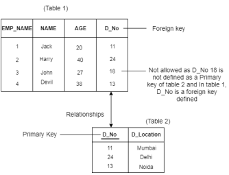
Referential integrity constraints work on the concept of Foreign Keys. A foreign key is a key attribute of a relation that can be referred in other relation.

Referential integrity constraint states that if a relation refers to a key attribute of a different or same relation, then that key element must exist.

Key takeaway

Relational data model is the primary data model, which is used widely around the world for data storage and processing. This model is simple and it has all the properties and capabilities required to process data with storage efficiency.

2.2 Schema-instance distinction

Database Schema

A database schema is the skeleton structure that represents the logical view of the entire database. It defines how the data is organized and how the relations among them are associated. It formulates all the constraints that are to be applied on the data.

A database schema defines its entities and the relationship among them. It contains a descriptive detail of the database, which can be depicted by means of schema diagrams. It’s the database designers who design the schema to help programmers understand the database and make it useful.

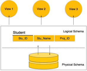
Fig 1 - Database schema

A database schema can be divided broadly into two categories −

Database Instance

It is important that we distinguish these two terms individually. Database schema is the skeleton of database. It is designed when the database doesn't exist at all. Once the database is operational, it is very difficult to make any changes to it. A database schema does not contain any data or information.

A database instance is a state of operational database with data at any given time. It contains a snapshot of the database. Database instances tend to change with time. A DBMS ensures that its every instance (state) is in a valid state, by diligently following all the validations, constraints, and conditions that the database designers have imposed.

Key takeaway

A database schema is the skeleton structure that represents the logical view of the entire database. It defines how the data is organized and how the relations among them are associated. It formulates all the constraints that are to be applied on the data.

A database schema defines its entities and the relationship among them. It contains a descriptive detail of the database, which can be depicted by means of schema diagrams. It’s the database designers who design the schema to help programmers understand the database and make it useful.

2.3 Referential integrity and foreign keys

Integrity Constraints

Types of Integrity Constraint

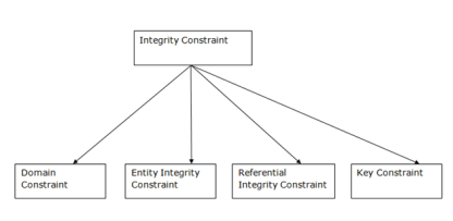
Fig 2 - Integrity Constraint

1. Domain constraints

Example:

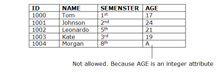
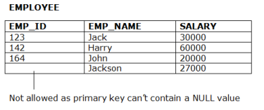
2. Entity integrity constraints

Example:

3. Referential Integrity Constraints

Example:

4. Key constraints

Example:

Foreign Key in DBMS

A foreign key is different from a super key, candidate key or primary key because a foreign key is the one that is used to link two tables together or create connectivity between the two.

Here, in this section, we will discuss foreign key, its use and look at some examples that will help us to understand the working and use of the foreign key. We will also see its practical implementation on a database, i.e., creating and deleting a foreign key on a table.

What is a Foreign Key

A foreign key is the one that is used to link two tables together via the primary key. It means the columns of one table points to the primary key attribute of the other table. It further means that if any attribute is set as a primary key attribute will work in another table as a foreign key attribute. But one should know that a foreign key has nothing to do with the primary key.

Use of Foreign Key

The use of a foreign key is simply to link the attributes of two tables together with the help of a primary key attribute. Thus, it is used for creating and maintaining the relationship between the two relations.

Example of Foreign Key

Let's discuss an example to understand the working of a foreign key.

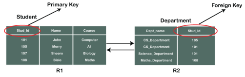
Consider two tables Student and Department having their respective attributes as shown in the below table structure:

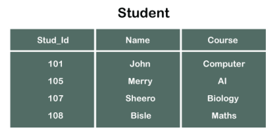
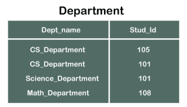
In the tables, one attribute, you can see, is common, that is Stud_Id, but it has different key constraints for both tables. In the Student table, the field Stud_Id is a primary key because it is uniquely identifying all other fields of the Student table. On the other hand, Stud_Id is a foreign key attribute for the Department table because it is acting as a primary key attribute for the Student table. It means that both the Student and Department table are linked with one another because of the Stud_Id attribute.

In the below-shown figure, you can view the following structure of the relationship between the two tables.

Creating Foreign Key constraint

On CREATE TABLE

Below is the syntax that will make us learn the creation of a foreign key in a table:

So, in this way, we can set a foreign key for a table in the MYSQL database.

In case of creating a foreign key for a table in SQL or Oracle server, the following syntax will work:

On ALTER TABLE

Following is the syntax for creating a foreign key constraint on ALTER TABLE:

Dropping Foreign Key

In order to delete a foreign key, there is a below-described syntax that can be used:

So, in this way, we can drop a foreign key using the ALTER TABLE in the MYSQL database.

Point to remember

When you drop the foreign key, one needs to take care of the integrity of the tables which are connected via a foreign key. In case you make changes in one table and disturbs the integrity of both tables, it may display certain errors due to improper connectivity between the two tables.

Referential Actions

There are some actions that are linked with the actions taken by the foreign key table holder:

1) Cascade

When we delete rows in the parent table (i.e., the one holding the primary key), the same columns in the other table (i.e., the one holding a foreign key) also gets deleted. Thus, the action is known as Cascade.

2) Set NULL

Such referential action maintains the referential integrity of both tables. When we manipulate/delete a referenced row in the parent/referenced table, in the child table (table having foreign key), the value of such referencing row is set as NULL. Such a referential action performed is known as Set NULL.

3) Set DEFAULT

Such an action takes place when the values in the referenced row of the parent table are updated, or the row is deleted, the values in the child table are set to default values of the column.

4) Restrict

It is the restriction constraint where the value of the referenced row in the parent table cannot be modified or deleted unless it is not referred by the foreign key in the child table. Thus, it is a normal referential action of a foreign key.

5) No Action

It is also a restriction constraint of the foreign key but is implemented only after trying to modify or delete the referenced row of the parent table.

6) Triggers

All these and other referential actions are basically implemented as triggers where the actions of a foreign key are much similar or almost similar to user-defined triggers. However, in some cases, the ordered referential actions get replaced by their equivalent user-defined triggers for ensuring proper trigger execution.

Key takeaway

2.4 Relational algebra

Relational algebra is a procedural query language. It gives a step by step process to obtain the result of the query. It uses operators to perform queries.

Types of Relational operation

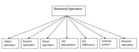
Fig 3 - Relational operation

1. Select Operation:

Where:

σ is used for selection prediction
r is used for relation
p is used as a propositional logic formula which may use connectors like: AND OR and NOT. These relational can use as relational operators like =, ≠, ≥, <, >, ≤.

For example: LOAN Relation

Input:

Output:

2. Project Operation:

Where

A1, A2, A3 is used as an attribute name of relation r.

Example: CUSTOMER RELATION

Input:

Output:

3. Union Operation:

A union operation must hold the following condition:

Example:

DEPOSITOR RELATION

BORROW RELATION

Input:

Output:

4. Set Intersection:

Example: Using the above DEPOSITOR table and BORROW table

Input:

Output:

5. Set Difference:

Example: Using the above DEPOSITOR table and BORROW table

Input:

Output:

6. Cartesian product

Example:

EMPLOYEE

DEPARTMENT

Input:

Output:

7. Rename Operation:

The rename operation is used to rename the output relation. It is denoted by rho (ρ).

Example: We can use the rename operator to rename STUDENT relation to STUDENT1.

Key takeaway

Relational algebra is a procedural query language. It gives a step by step process to obtain the result of the query. It uses operators to perform queries.

2.5 Various types of joins

A Join operation combines related tuples from different relations, if and only if a given join condition is satisfied. It is denoted by ⋈.

Example:

EMPLOYEE

SALARY

Result:

Types of Join operations:

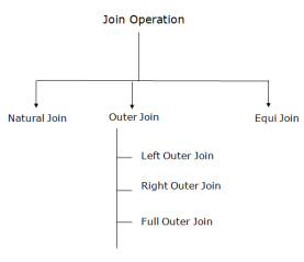
Fig 4 – Join Operation

1. Natural Join:

Example: Let's use the above EMPLOYEE table and SALARY table:

Input:

Output:

2. Outer Join:

The outer join operation is an extension of the join operation. It is used to deal with missing information.

Example:

EMPLOYEE

FACT_WORKERS

Input:

Output:

An outer join is basically of three types:

a. Left outer join:

Example: Using the above EMPLOYEE table and FACT_WORKERS table

Input:

b. Right outer join:

Example: Using the above EMPLOYEE table and FACT_WORKERS Relation

Input:

Output:

c. Full outer join:

Example: Using the above EMPLOYEE table and FACT_WORKERS table

Input:

Output:

3. Equijoin:

It is also known as an inner join. It is the most common join. It is based on matched data as per the equality condition. The equi join uses the comparison operator(=).

Example:

CUSTOMER RELATION

PRODUCT

Input:

Output:

Key takeaway

A Join operation combines related tuples from different relations, if and only if a given join condition is satisfied.

2.6 Tuple relation calculus

Relational Calculus

Types of Relational calculus:

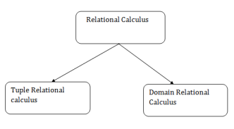
Fig 5 - Relational calculus

1. Tuple Relational Calculus (TRC)

Notation:

Where

T is the resulting tuples

P(T) is the condition used to fetch T.

For example:

OUTPUT: This query selects the tuples from the AUTHOR relation. It returns a tuple with 'name' from Author who has written an article on 'database'.

TRC (tuple relation calculus) can be quantified. In TRC, we can use Existential (∃) and Universal Quantifiers (∀).

For example:

Output: This query will yield the same result as the previous one.

2. Domain Relational Calculus (DRC)

Notation:

Where

a1, a2 are attributes
P stands for formula built by inner attributes

For example:

Output: This query will yield the article, page, and subject from the relational javatpoint, where the subject is a database.

Key takeaway

2.7 Example queries

Types of SQL Commands

There are five types of SQL commands: DDL, DML, DCL, TCL, and DQL.

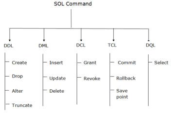
Fig 5 – SQL Commands

1. Data Definition Language (DDL)

Here are some commands that come under DDL:

a. CREATE It is used to create a new table in the database.

Syntax:

Example:

b. DROP: It is used to delete both the structure and record stored in the table.

Syntax

Example

c. ALTER: It is used to alter the structure of the database. This change could be either to modify the characteristics of an existing attribute or probably to add a new attribute.

Syntax:

To add a new column in the table

To modify existing column in the table:

EXAMPLE

d. TRUNCATE: It is used to delete all the rows from the table and free the space containing the table.

Syntax:

Example:

2. Data Manipulation Language

Here are some commands that come under DML:

a. INSERT: The INSERT statement is a SQL query. It is used to insert data into the row of a table.

Syntax:

Or

For example:

b. UPDATE: This command is used to update or modify the value of a column in the table.

Syntax:

For example:

c. DELETE: It is used to remove one or more row from a table.

Syntax:

For example:

3. Data Control Language

DCL commands are used to grant and take back authority from any database user.

Here are some commands that come under DCL:

a. Grant: It is used to give user access privileges to a database.

Example

b. Revoke: It is used to take back permissions from the user.

Example

4. Transaction Control Language

TCL commands can only use with DML commands like INSERT, DELETE and UPDATE only.

These operations are automatically committed in the database that's why they cannot be used while creating tables or dropping them.

Here are some commands that come under TCL:

a. Commit: Commit command is used to save all the transactions to the database.

Syntax:

Example:

b. Rollback: Rollback command is used to undo transactions that have not already been saved to the database.

Syntax:

Example:

c. SAVEPOINT: It is used to roll the transaction back to a certain point without rolling back the entire transaction.

Syntax:

5. Data Query Language

DQL is used to fetch the data from the database.

It uses only one command:

a. SELECT: This is the same as the projection operation of relational algebra. It is used to select the attribute based on the condition described by WHERE clause.

Syntax:

For example:

Key takeaway

2.8 Introduction to SQL

SQL

Rules:

SQL follows the following rules:

SQL process:

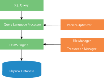
Fig 6 - SQL process

Characteristics of SQL

Advantages of SQL

There are the following advantages of SQL:

High speed

Using the SQL queries, the user can quickly and efficiently retrieve a large amount of records from a database.

No coding needed

In the standard SQL, it is very easy to manage the database system. It doesn't require a substantial amount of code to manage the database system.

Well defined standards

Long established are used by the SQL databases that are being used by ISO and ANSI.

Portability

SQL can be used in laptop, PCs, server and even some mobile phones.

Interactive language

SQL is a domain language used to communicate with the database. It is also used to receive answers to the complex questions in seconds.

Multiple data view

Using the SQL language, the users can make different views of the database structure.

Key takeaway

2.9 Data definition statements with constraints

Constraints are the rules enforced on the data columns of a table. These are used to limit the type of data that can go into a table. This ensures the accuracy and reliability of the data in the database.

Constraints could be either on a column level or a table level. The column level constraints are applied only to one column, whereas the table level constraints are applied to the whole table.

Following are some of the most commonly used constraints available in SQL.

NOT NULL Constraint − Ensures that a column cannot have NULL value.

Constraints can be specified when a table is created with the CREATE TABLE statement or you can use the ALTER TABLE statement to create constraints even after the table is created.

Dropping Constraints

Any constraint that you have defined can be dropped using the ALTER TABLE command with the DROP CONSTRAINT option.

For example, to drop the primary key constraint in the EMPLOYEES table, you can use the following command.

ALTER TABLE EMPLOYEES DROP CONSTRAINT EMPLOYEES_PK;

Some implementations may provide shortcuts for dropping certain constraints. For example, to drop the primary key constraint for a table in Oracle, you can use the following command.

ALTER TABLE EMPLOYEES DROP PRIMARY KEY;

Some implementations allow you to disable constraints. Instead of permanently dropping a constraint from the database, you may want to temporarily disable the constraint and then enable it later.

Integrity Constraints

Integrity constraints are used to ensure accuracy and consistency of the data in a relational database. Data integrity is handled in a relational database through the concept of referential integrity.

There are many types of integrity constraints that play a role in Referential Integrity (RI). These constraints include Primary Key, Foreign Key, Unique Constraints and other constraints which are mentioned above.

Key takeaway

Constraints are the rules enforced on the data columns of a table. These are used to limit the type of data that can go into a table. This ensures the accuracy and reliability of the data in the database.

Constraints could be either on a column level or a table level. The column level constraints are applied only to one column, whereas the table level constraints are applied to the whole table.

2.10 Update behaviours

The SQL UPDATE statement is used to modify the data that is already in the database. The condition in the WHERE clause decides that which row is to be updated.

Syntax

Sample Table

EMPLOYEE

Updating single record

Update the column EMP_NAME and set the value to 'Emma' in the row where SALARY is 500000.

Syntax

Query

Output: After executing this query, the EMPLOYEE table will look like:

Updating multiple records

If you want to update multiple columns, you should separate each field assigned with a comma. In the EMPLOYEE table, update the column EMP_NAME to 'Kevin' and CITY to 'Boston' where EMP_ID is 5.

Syntax

Query

Output

Without use of WHERE clause

If you want to update all row from a table, then you don't need to use the WHERE clause. In the EMPLOYEE table, update the column EMP_NAME as 'Harry'.

Syntax

Query

Output

Key takeaway

The SQL UPDATE statement is used to modify the data that is already in the database. The condition in the WHERE clause decides that which row is to be updated.

Syntax

2.11 Nested Queries

SQL Sub Query

A Subquery is a query within another SQL query and embedded within the WHERE clause.

Important Rule:

1. Subqueries with the Select Statement

SQL subqueries are most frequently used with the Select statement.

Syntax

Example

Consider the EMPLOYEE table have the following records:

The subquery with a SELECT statement will be:

This would produce the following result:

2. Subqueries with the INSERT Statement

Syntax:

Example

Consider a table EMPLOYEE_BKP with similar as EMPLOYEE.

Now use the following syntax to copy the complete EMPLOYEE table into the EMPLOYEE_BKP table.

3. Subqueries with the UPDATE Statement

The subquery of SQL can be used in conjunction with the Update statement. When a subquery is used with the Update statement, then either single or multiple columns in a table can be updated.

Syntax

Example

Let's assume we have an EMPLOYEE_BKP table available which is backup of EMPLOYEE table. The given example updates the SALARY by .25 times in the EMPLOYEE table for all employee whose AGE is greater than or equal to 29.

This would impact three rows, and finally, the EMPLOYEE table would have the following records.

4. Subqueries with the DELETE Statement

The subquery of SQL can be used in conjunction with the Delete statement just like any other statements mentioned above.

Syntax

Example

Let's assume we have an EMPLOYEE_BKP table available which is backup of EMPLOYEE table. The given example deletes the records from the EMPLOYEE table for all EMPLOYEE whose AGE is greater than or equal to 29.

This would impact three rows, and finally, the EMPLOYEE table would have the following records.

Key takeaway

A Subquery is a query within another SQL query and embedded within the WHERE clause.

Important Rule:

2.12 Aggregate functions group by and having clauses

What is the SQL Group by Clause?

The GROUP BY clause is a SQL command that is used to group rows that have the same values. The GROUP BY clause is used in the SELECT statement. Optionally it is used in conjunction with aggregate functions to produce summary reports from the database.

That's what it does, summarizing data from the database.

The queries that contain the GROUP BY clause are called grouped queries and only return a single row for every grouped item.

SQL GROUP BY Syntax

Now that we know what the SQL GROUP BY clause is, let's look at the syntax for a basic group by query.

SELECT statements... GROUP BY column_name1[,column_name2,...] [HAVING condition];

HERE

Grouping using a Single Column

In order to help understand the effect of SQL Group By clause, let's execute a simple query that returns all the gender entries from the members table.

SELECT gender FROM members ;

Suppose we want to get the unique values for genders. We can use a following query -

SELECT gender FROM members GROUP BY gender;

Executing the above script in MYSQL workbench against the Myflixdb gives us the following results.

Note only two results have been returned. This is because we only have two gender types Male and Female. The GROUP BY clause in SQL grouped all the "Male" members together and returned only a single row for it. It did the same with the "Female" members.

Grouping using multiple columns

Suppose that we want to get a list of movie category_id  and corresponding years in which they were released.

Let's observe the output of this simple query

SELECT category_id,year_released FROM movies ;

The above result has many duplicates.

Let's execute the same query using group by in SQL -

SELECT category_id,year_released FROM movies GROUP BY category_id,year_released;

Executing the above script in MySQL workbench against the myflixdb gives us the following results shown below.

The GROUP BY clause operates on both the category id and year released to identify unique rows in our above example.

If the category id is the same but the year released is different, then a row is treated as a unique one .If the category id and the year released is the same for more than one row, then it's considered a duplicate and only one row is shown.

Grouping and aggregate functions

Suppose we want total number of males and females in our database. We can use the following script shown below to do that.

SELECT gender,COUNT(membership_number)  FROM members GROUP BY gender;

Executing the above script in MySQL workbench against the myflixdb gives us the following results.

The results shown below are grouped by every unique gender value posted and the number of grouped rows is counted using the COUNT aggregate function.

Restricting query results using the HAVING clause

It's not always that we will want to perform groupings on all the data in a given table. There will be times when we will want to restrict our results to a certain given criteria.  In such cases , we can use the HAVING clause

Suppose we want to know all the release years for movie category id 8. We would use the following script to achieve our results.

SELECT * FROM movies GROUP BY category_id,year_released HAVING category_id = 8;

Executing the above script in MySQL workbench against the Myflixdb gives us the following results shown below.

Note only movies with category id 8 have been affected by our GROUP BY clause.

Summary

Key takeaway

The GROUP BY clause is a SQL command that is used to group rows that have the same values. The GROUP BY clause is used in the SELECT statement. Optionally it is used in conjunction with aggregate functions to produce summary reports from the database.

That's what it does, summarizing data from the database.

The queries that contain the GROUP BY clause are called grouped queries and only return a single row for every grouped item.

Reference Books

1. “Database Management Systems”, Raghu Ramakrishnan and Johannes Gehrke, 2002, 3rd Edition.

2. “Fundamentals of Database Systems”, RamezElmasri and ShamkantNavathe, Benjamin Cummings, 1999, 3rd Edition.

3. “Database System Concepts”, Abraham Silberschatz, Henry F. Korth and S.Sudarshan, Mc Graw Hill, 2002, 4th Edition.