Unit - 2
Algorithm Analysis
Time complexity:
The time complexity of an algorithm is the amount of time required to complete the execution. The time complexity of an algorithm is denoted by the big O notation. Here, big O notation is the asymptotic notation to represent the time complexity. The time complexity is mainly calculated by counting the number of steps to finish the execution.
Let's understand the time complexity through an example.
- Sum=0;
- // Suppose we have to calculate the sum of n numbers.
- For i=1 to n
- Sum=sum+i;
- // when the loop ends then sum holds the sum of the n numbers
- Return sum;
In the above code, the time complexity of the loop statement will be at least n, and if the value of n increases, then the time complexity also increases. While the complexity of the code, i.e., return sum will be constant as its value is not dependent on the value of n and will provide the result in one step only. We generally consider the worst-time complexity as it is the maximum time taken for any given input size.
Space complexity:
An algorithm's space complexity is the amount of space required to solve a problem and produce an output. Similar to the time complexity, space complexity is also expressed in big O notation.
For an algorithm, the space is required for the following purposes:
- To store program instructions
- To store constant values
- To store variable values
To track the function calls, jumping statements, etc.
Key takeaway
The time complexity of an algorithm is the amount of time required to complete the execution.
An algorithm's space complexity is the amount of space required to solve a problem and produce an output.
Big Oh (O) Notation:
- It is the formal way to express the time complexity.
- It is used to define the upper bound of an algorithm’s running time.
- It shows the worst-case time complexity or largest amount of time taken by the algorithm to perform a certain task.
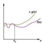
Fig: Big Oh notation
Here, f (n) <= g (n) …………….(eq1)
where n>= k, C>0 and k>=1
If any algorithm satisfies the eq1 condition then it becomes f (n)= O (g (n))
Big Omega (ῼ) Notation
- It is the formal way to express the time complexity.
- It is used to define the lower bound of an algorithm’s running time.
- It shows the best-case time complexity or best of time taken by the algorithm to perform a certain task.
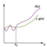
Fig: Big omega notation
Here, f (n) >= g (n)
Where n>=k and c>0, k>=1
If any algorithm satisfies the eq1 condition then it becomes f (n)= ῼ (g (n))
Theta (Θ) Notation
- It is the formal way to express the time complexity.
- It is used to define the lower as well as upper bound of an algorithm’s running time.
- It shows the average case time complexity or average of time taken by the algorithm to perform a certain task.
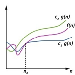
Fig: Theta notation
Let C1 g(n) be upper bound and C2 g(n) be lower bound.
C1 g(n)<= f (n)<=C2 g(n)
Where C1, C2>0 and n>=k
Key takeaway
- Big Oh is used to define the upper bound of an algorithm’s running time.
- Big Omega is used to define the lower bound of an algorithm’s running time.
- Theta is used to define the lower as well as upper bound of an algorithm’s running time.
Linear search
Searching is the process of looking for a certain item in a list. If the element is found in the list, the process is considered successful, and the location of that element is returned; otherwise, the search is considered unsuccessful.
Linear Search and Binary Search are two prominent search strategies. So, we'll talk about a popular search strategy called the Linear Search Algorithm.
The linear search algorithm is also known as the sequential search algorithm. It is the most basic search algorithm. We just traverse the list in linear search and match each element of the list with the object whose position has to be discovered. If a match is found, the algorithm delivers the item's location; otherwise, NULL is returned.
It's commonly used to find an element in an unordered list, or one in which the items aren't sorted. The time complexity of linear search in the worst-case scenario is O(n).
The following are the steps involved in implementing Linear Search:
● We must first use a for loop to traverse the array elements.
● Compare the search element with the current array element in each iteration of the for loop, and -
● Return the index of the related array entry if the element matches.
● If the element you're looking for doesn't match, move on to the next one.
● Return -1 if there is no match or the search element is not found in the given array.
Let's look at the linear search algorithm now.
Algorithm
Linear_Search(a, n, val) // 'a' is the given array, 'n' is the size of given array, 'val' is the value to search
Step 1: set pos = -1
Step 2: set i = 1
Step 3: repeat step 4 while i <= n
Step 4: if a[i] == val
Set pos = i
Print pos
Go to step 6
[end of if]
Set ii = i + 1
[end of loop]
Step 5: if pos = -1
Print "value is not present in the array "
[end of if]
Step 6: exit
Time Complexity
Case | Time Complexity |
Best Case | O(1) |
Average Case | O(n) |
Worst Case | O(n) |
Space Complexity
Space Complexity | O(1) |
Application of Linear Search Algorithm
The linear search algorithm is useful for the following tasks:
● Both single-dimensional and multi-dimensional arrays can benefit from linear search.
● When the array has only a few elements, linear search is simple to implement and effective.
● When performing a single search in an unordered-List, Linear Search is also quite efficient.
Binary Search
Binary search is the search technique which works efficiently on the sorted lists. Hence, in order to search an element into some list by using binary search technique, we must ensure that the list is sorted.
Binary search follows a divide and conquer approach in which the list is divided into two halves and the item is compared with the middle element of the list. If the match is found then, the location of the middle element is returned; otherwise, we search into either of the halves depending upon the result produced through the match.
Binary search algorithm is given below.
BINARY_SEARCH(A, lower_bound, upper_bound, VAL)
● Step 1: [INITIALIZE] SET BEG = lower_bound
END = upper_bound, POS = - 1
● Step 2: Repeat Steps 3 and 4 while BEG <=END
● Step 3: SET MID = (BEG + END)/2
● Step 4: IF A[MID] = VAL
SET POS = MID
PRINT POS
Go to Step 6
ELSE IF A[MID] > VAL
SET END = MID – 1
ELSE
SET BEG = MID + 1
[END OF IF]
[END OF LOOP]
● Step 5: IF POS = -1
PRINT "VALUE IS NOT PRESENT IN THE ARRAY"
[END OF IF]
● Step 6: EXIT
Complexity
SN | Performance | Complexity |
1 | Worst case | O(log n) |
2 | Best case | O(1) |
3 | Average Case | O(log n) |
4 | Worst case space complexity | O(1) |
Example
Let us consider an array arr = {1, 5, 7, 8, 13, 19, 20, 23, 29}. Find the location of the item 23 in the array.
In 1st step:
- BEG = 0
- END = 8ron
- MID = 4
- a[mid] = a[4] = 13 < 23, therefore
In Second step:
- Beg = mid +1 = 5
- End = 8
- Mid = 13/2 = 6
- a[mid] = a[6] = 20 < 23, therefore;
In third step:
- Beg = mid + 1 = 7
- End = 8
- Mid = 15/2 = 7
- a[mid] = a[7]
- a[7] = 23 = item;
- Therefore, set location = mid;
- The location of the item will be 7.
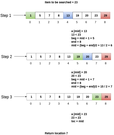
Fig - Example
Bubble sort
Bubble Sort is a simple algorithm for sorting a collection of n elements that is provided in the form of an array with n elements. Bubble Sort compares each element individually and sorts them according to their values.
If an array must be sorted in ascending order, bubble sort will begin by comparing the first and second members of the array, swapping both elements if the first element is greater than the second, and then moving on to compare the second and third elements, and so on.
If there are n elements in total, we must repeat the method n-1 times.
It's called bubble sort because the largest element in the given array bubbles up to the last position or highest index with each full iteration, similar to how a water bubble rises to the sea surface.
Although it is simple to use, bubble sort is largely employed as an educational tool because its performance in the actual world is low. It isn't designed to handle huge data collections. Bubble sort has an average and worst-case complexity of O(n2), where n is the number of elements.
Sorting is done by going through all of the items one by one, comparing them to the next closest element, and swapping them if necessary.
Algorithm
Assume that arr is an array of n elements in the algorithm below. The algorithm's presumed swap function will swap the values of specified array members.
Begin BubbleSort(arr)
for all array elements
if arr[i] > arr[i+1]
swap(arr[i], arr[i+1])
end if
end for
return arr
End BubbleSort
Working of Bubble Sort
Assume we're attempting to arrange the elements in ascending order.
1. First Iteration (Compare and Swap)
● Compare the first and second elements starting with the first index.
● The first and second elements are swapped if the first is bigger than the second.
● Compare and contrast the second and third elements now. If they aren't in the right order, swap them.
● The process continues until the last piece is added.
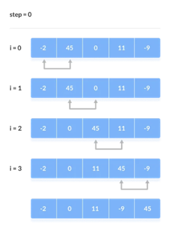
2. Remaining Iteration
For the remaining iterations, the same procedure is followed.
The largest element among the unsorted items is placed at the conclusion of each iteration.
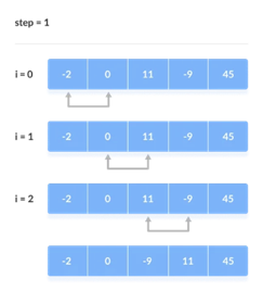
The comparison takes place up to the last unsorted element in each iteration.
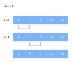
When all of the unsorted elements have been placed in their correct placements, the array is said to be sorted.

Bubble sort in C++
To use bubble sort to sort an array in ascending order in C++ programming, you must first ask the user for the array size and entries. Now, using the bubble sort technique, sort the array items and display the sorted array on the screen as demonstrated in the following software.
#include<iostream>
Using namespace std;
Int main()
{
int n, i, arr[50], j, temp;
cout<<"Enter the Size (max. 50): ";
cin>>n;
cout<<"Enter "<<n<<" Numbers: ";
for(i=0; i<n; i++)
cin>>arr[i];
cout<<"\nSorting the Array using Bubble Sort Technique..\n";
for(i=0; i<(n-1); i++)
{
for(j=0; j<(n-i-1); j++)
{
if(arr[j]>arr[j+1])
{
temp = arr[j];
arr[j] = arr[j+1];
arr[j+1] = temp;
}
}
}
cout<<"\nArray Sorted Successfully!\n";
cout<<"\nThe New Array is: \n";
for(i=0; i<n; i++)
cout<<arr[i]<<" ";
cout<<endl;
return 0;
}
Sample run
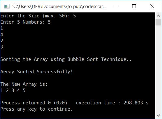
Key takeaway
- Compare and swap adjacent elements of the list if they are out of order.
- After repeating the procedure, we end up 'bubbling up' the largest element to the last place on the list by doing it repeatedly.
Insertion sort
Insertion style is a decrease & conquer technique application. It is a sort based on comparison in which the sorted array is constructed on one entry at a time.
Insertion sorting is a very basic process for sorting numbers in an ascending or descending order. The gradual method is accompanied by this method. It can be contrasted with the method of sorting cards at the time of playing a game.
The numbers that are needed to be sorted are known as keys. Here is the insertion sort method algorithm.
Algorithm:
Algorithm: Insertion-Sort (A)
For j = 2 to A.length
Key = A[j]
// Insert A[j] into the sorted sequence A[1.. j - 1]
i = j - 1
While i > 0 and A[i] > key
A[i + 1] = A[i]
i = i -1
A[i + 1] = key
Analysis:
This algorithm's run time is very dependent on the input given.
If the numbers given are sorted, this algorithm runs in O(n) time. If the numbers given are in reverse order, the algorithm runs in O(n2) time.
Example:
Using insertion sort to sort the following list of elements:
89, 45, 68, 90, 29, 34, 17
89 |45 68 90 29 34 17
45 89 |68 90 29 34 17
45 68 89 |90 29 34 17
45 68 89 90 |29 34 17
29 45 68 89 90 |34 17
29 34 45 68 89 90 |17
17 29 34 45 68 89 90
Application:
In the following instances, the insertion sort algorithm is used:
- When only a few elements are in the list.
- When there are few elements for sorting.
Advantages:
- Straightforward implementation. Three variants exist.
● Left to right scan
● Right to left scan
● Binary insertion sort
2. Effective on a small list of components, on a nearly sorted list.
3. In the best example, running time is linear.
4. This algorithm is stable.
5. Is the on-the-spot algorithm
Example code in C++
#include<iostream>
Using namespace std;
Void display(int *array, int size) {
for(int i = 0; i<size; i++)
cout << array[i] << " ";
cout << endl;
}
Void insertionSort(int *array, int size) {
int key, j;
for(int i = 1; i<size; i++) {
key = array[i];//take value
j = i;
while(j > 0 && array[j-1]>key) {
array[j] = array[j-1];
j--;
}
array[j] = key; //insert in right place
}
}
Int main() {
int n;
cout << "Enter the number of elements: ";
cin >> n;
int arr[n]; //create an array with given number of elements
cout << "Enter elements:" << endl;
for(int i = 0; i<n; i++) {
cin >> arr[i];
}
cout << "Array before Sorting: ";
display(arr, n);
insertionSort(arr, n);
cout << "Array after Sorting: ";
display(arr, n);
}
Output
Enter the number of elements: 6
Enter elements:
9 45 23 71 80 55
Array before Sorting: 9 45 23 71 80 55
Array after Sorting: 9 23 45 55 71 80
Key takeaways
- Insertion sorting is a very basic process for sorting numbers in an ascending or descending order.
- Insertion style is a decrease & conquer technique application.
- It is a sort based on comparison in which the sorted array is constructed on one entry at a time.
Selection sort
In the selection sort, the smallest value among the array's unsorted items is chosen in each pass and inserted into the proper spot.
To begin, locate the array's smallest element and set it in the first position. Then locate the array's second smallest element and set it in the second spot. The procedure is repeated till the sorted array is obtained.
The n-1 pass of the selection sort algorithm is used to sort the array of n entries.
● The smallest element of the array, as well as its index pos, must be identified in the first run. Swap A[0] and A[pos] after that. As a result of sorting A[0], we now have n -1 elements to sort.
● The location pos of the smallest element in the sub-array A[n-1] is obtained in the second pass. Swap A[1] and A[pos] after that. After sorting A[0] and A[1], we're left with n-2 unsorted elements.
● The position pos of the smaller element between A[n-1] and A[n-2] must be found in the n-1st pass. Swap A[pos] and A[n-1] after that.
As a result, the items A[0], A[1], A[2],...., A[n-1] are sorted using the procedure described above.
Example
Consider the following six-element array. Using selection sort, sort the array's elements.
A = {10, 2, 3, 90, 43, 56}.
Pass | Pos | A[0] | A[1] | A[2] | A[3] | A[4] | A[5] |
1 | 1 | 2 | 10 | 3 | 90 | 43 | 56 |
2 | 2 | 2 | 3 | 10 | 90 | 43 | 56 |
3 | 2 | 2 | 3 | 10 | 90 | 43 | 56 |
4 | 4 | 2 | 3 | 10 | 43 | 90 | 56 |
5 | 5 | 2 | 3 | 10 | 43 | 56 | 90 |
Sorted A = {2, 3, 10, 43, 56, 90}
Algorithm
SELECTION SORT(ARR, N)
● Step 1: Repeat Steps 2 and 3 for K = 1 to N-1
● Step 2: CALL SMALLEST(ARR, K, N, POS)
● Step 3: SWAP A[K] with ARR[POS]
[END OF LOOP]
● Step 4: EXIT
SMALLEST (ARR, K, N, POS)
● Step 1: [INITIALIZE] SET SMALL = ARR[K]
● Step 2: [INITIALIZE] SET POS = K
● Step 3: Repeat for J = K+1 to N -1
IF SMALL > ARR[J]
SET SMALL = ARR[J]
SET POS = J
[END OF IF]
[END OF LOOP]
● Step 4: RETURN POS
Example code in C++
#include<iostream>
Using namespace std;
Void swapping(int &a, int &b) { //swap the content of a and b
int temp;
temp = a;
a = b;
b = temp;
}
Void display(int *array, int size) {
for(int i = 0; i<size; i++)
cout << array[i] << " ";
cout << endl;
}
Void selectionSort(int *array, int size) {
int i, j, imin;
for(i = 0; i<size-1; i++) {
imin = i; //get index of minimum data
for(j = i+1; j<size; j++)
if(array[j] < array[imin])
imin = j;
//placing in correct position
swap(array[i], array[imin]);
}
}
Int main() {
int n;
cout << "Enter the number of elements: ";
cin >> n;
int arr[n]; //create an array with given number of elements
cout << "Enter elements:" << endl;
for(int i = 0; i<n; i++) {
cin >> arr[i];
}
cout << "Array before Sorting: ";
display(arr, n);
selectionSort(arr, n);
cout << "Array after Sorting: ";
display(arr, n);
}
Output
Enter the number of elements: 6
Enter elements:
5 9 7 23 78 20
Array before Sorting: 5 9 7 23 78 20
Array after Sorting: 5 7 9 20 23 78
Key takeaway
- In the selection sort, the smallest value among the array's unsorted items is chosen in each pass and inserted into the proper spot.
- To begin, locate the array's smallest element and set it in the first position.
- Then locate the array's second smallest element and set it in the second spot.
References:
- Data structure through C++- Yashwant Kanitkar (BPB Publications)
- Principles of Data structures using c++ - Vinu V. Das(New Age International Publication)
- Data Structures with C- SEYMOUR LIPSCHUTZ( Tata McGraw-Hill)
- Data structures, Algorithms and Applications in C++, S.Sahni, University Press (India) Pvt.Ltd, 2nd edition, Universities Press Orient Longman Pvt. Ltd.